
The unwanted sum signal at the output of the mixer is removed by means of a lowpass filter, so that only the difference signal remains. The low frequency signal component filtered in this way generates a time-dependent voltage v(t) whose maximum amplitude is determined by the scaling factor of the phase detector constant KD. In general, KD is device-dependent and has no influence on the calculation of the phase noise L(f).
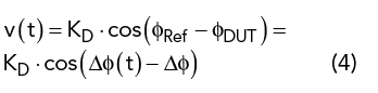
Considering the small-angle approximation cos(∝)≈∝ for ∝<<1, Equation (4) can be simplified, assuming a mean phase difference of  .
.

The output voltage v(t) of the phase comparator is evaluated as a measure of the phase changes in the time domain. The calculation of the single sideband phase noise L(f) is performed by means of an FFT in the frequency domain. If the reference oscillator has the same phase noise characteristics as the test oscillator, the measurement result must be corrected by -3 dB (factor of 0.5), since the uncorrelated noise powers of both oscillators add up. If the reference oscillator has a better phase noise by at least one decade, no correction is necessary.
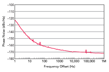
Figure 3 Phase noise measurement of an ultra-low phase noise oscillator with a carrier frequency of 10 MHz.
Figure 3 is an example of a phase noise measurement of an ultra-low phase noise oscillator from KVG Quartz Crystal Technology with a carrier frequency of 10 MHz. The measurement was performed with a Holzworth phase noise analyzer with a measurement time of 1 hour. Both the near-carrier phase noise with a value of -122.5 dBc/Hz at 1 Hz offset and the phase noise of -169 dBc/Hz at 10 kHz show the limits of what is physically feasible.
A standard oven-controlled crystal oscillator (OXCO) at the same frequency has about 20 dBc/Hz worse phase noise at 1 Hz carrier offset than an ultra-low phase noise oscillator. Phase noise measurements are strongly sensitive with respect to mechanical or electromagnetic disturbances originating from the environment of the measurement setup. In Figure 3, small disturbances of the phase noise measurement can be observed, for example, at 50 Hz (mains frequency household current) and 16.7 Hz (mains frequency of the German railway), which can be further minimized by suitable mains filters of the measurement equipment and the control voltage of the oscillator.
JITTER
In addition to phase noise, jitter is another representation of the deviation of the phase angle of a periodic signal. It can be graphically interpreted as the time deviation of a signal from its ideal position over a series of signal periods. With an ideal measuring device (infinite time resolution and no inherent noise), one could look at individual clock edges and derive a jitter value via an absolute time measurement. This is not possible, however, even with the best measuring devices available.
In practice, the jitter measurement is often derived from the phase noise measurement, previously described, and will be explained in more detail later. For a direct jitter measurement, a measurement by means of a so-called “eye diagram” is used, in which the measurement is performed relative to a reference edge.
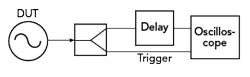
Figure 4 Jitter measurement using a delayed signal.
The eye diagram consists of a superposition of many sections from the signal curve to be measured. An exemplary measurement setup is shown in Figure 4. The signal from the DUT is split by a splitter with one signal path fed through a delay line whose delay is greater than the period of the signal. The non-delayed signal serves as a trigger and the delayed signal is applied to the input of the oscilloscope. This results in the phase shift always being measured relative to one of the preceding signal edges. By superimposing a large number of these measurements, a quantitative value of the jitter magnitude can be determined from the “opening of the eye diagram” by means of statistical analysis.
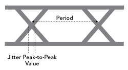
Figure 5 Deriving jitter from the eye diagram.
Figure 5 is an example of an eye diagram. Due to the intrinsic signal trigger, the signal edges are mapped on top of each other according to their phase shifts. From the superposition of several oscillation periods, quantities such as the average period duration and jitter can be determined. From the width of the signal distribution at zero crossing, a quantitative value for the jitter can be calculated on a statistical basis. In this example, the peak-to-peak value of the jitter is shown as the maximum expansion of the signal curve.
This measurement method is limited by the noise of the oscilloscope below the frequency range f = 1/(2 π τd), where τd is the length of the delay line. Below this cutoff frequency, the sensitivity drops by about 20 dB per decade. Thus, this method is well suited for jitter measurements at frequencies far from the carrier, for example the sidebands.
The noise in oscillators is basically a superposition of stochastic processes. The peak value is therefore usually specified on a purely statistical basis using a Gaussian distribution as the distribution function. This results in a crest factor (ratio of peak value to RMS value) of 3 between the peak and RMS value, or factor of 6 between the peak-to-peak and RMS value. The maximum jitter amplitude is with a probability of 99.7 percent (deviation in the interval ±3σ) within the statistical limits of the specified peak-to-peak value. When measuring and specifying jitter, it is important to note whether the specification is expressed as the effective value (RMS), peak value (peak) or peak-to-peak value (peak-to-peak).