
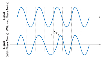
Figure 1 Random, time-dependent phase error (Δφ) in the sinusoidal signal.
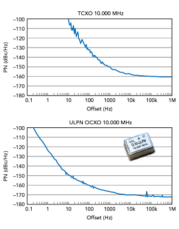
Figure 2 Phase noise diagrams for a KVG Quartz Crystal Technology TCXO and an ultra-low phase noise OCXO.

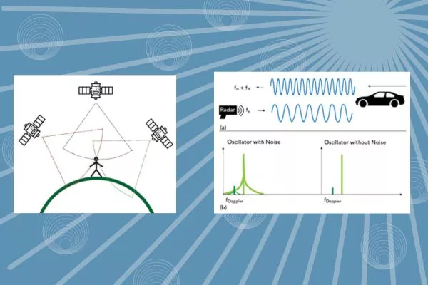
Figure 3 (a) Principle of signal mixing in a network analyzer. (b) Effects of mixing an input signal with a noisy LO signal. Source: Revised with permission from Rohde & Schwarz.
In most areas of our daily lives, data collection and processing, along with large parts of the critical infrastructure have been digitized. Common to all of these efforts is the need for highly accurate reference clocks. Often, crystal oscillators of various designs are used as frequency-determining components. These devices range from simple, unregulated crystal oscillators (XO/VCXOs) to temperature-compensated oscillators (TCXOs) and heated crystal oscillators (OCXOs). One of the most important quality criteria for high performance is the frequency stability of the quartz oscillators. Frequency stability on short time scales can be described by the three quantities: phase noise, jitter and short-term stability. A comprehensive compilation of these three measurement quantities and their interrelationships was published in the January 2023 issue of Microwave Journal.
After a short overview of important terms, this article will address the applications of high precision quartz oscillators. Case studies from the fields of measurement technology, data transmission, navigation, radar technology and the processing of audio signals will be considered in detail. In addition to the necessity of extremely low phase noise, the effects of poor phase noise performance are explained for the individual areas.
PHASE NOISE BASICS
Noise effects in electrical circuits are a ubiquitous phenomenon that can be attributed to various physical causes. The noise near the carrier is largely determined by the quality of the oscillator crystal, which acts as a narrowband filter in the range of the resonant frequency in the oscillator circuit. Figure 1 shows the short-term frequency instabilities that show up in the time domain as a deviation of the zero crossings (phase position) of the actual signal waveform compared to the ideal sinusoid. A modulation of the amplitude is not shown in this figure.
The most important parameters describing phase fluctuations are the phase noise, L(f), the jitter, ΔT(Δf), and the short time stability:  Figure 2 shows the phase noise plots of a good TCXO and a very good ultra-low phase noise (ULPN) OCXO from KVG Quartz Crystal Technology. “Good” 10 MHz TCXOs achieve phase noise as low as -100 dBc/Hz at 10 Hz offset frequency and a noise floor of -160 dBc/Hz at 100 kHz offset. “Good” ULPN 10 MHz OCXOs are available today with a phase noise of -123 dBc/Hz already at 1 Hz offset and -149 dBc/Hz at 10 Hz offset with a noise floor of better than -170 dBc/Hz.
The short-term stability, mostly expressed in the form of the “Allan Variance” or “Allan Deviation” (ADEV), is much better for good OCXOs than for good TCXOs. “Good” 10 MHz TCXOs have an ADEV in the range of 2 × 10⁻¹⁰ to 2 × 10-11 for a τ of 1 sec. “Good” 10 MHz OCXOs have an ADEV of 2 × 10-12 to 2 × 10-13, which is about two decades better.
MEASUREMENT TECHNOLOGY APPLICATIONS
Especially in the high frequency range, measurement technology relies on the fact that a signal to be measured is converted to a different and usually lower frequency by mixing with another signal. Low frequency signals are generally easier to analyze and fixed frequency filters and amplifiers can be used to measure the device. The signal to be measured is mixed down to the required frequency range using a local oscillator inside the device.
Figure 3a shows the basic principle of signal mixing in simplified form. In the mixer element, the input signal fin is mixed with the signal of a local oscillator fLO, forming a superposition of the difference signal, |fLO-fin| and the sum signal, fin+fLO. If the local oscillator has a phase noise that cannot be neglected, this noise characteristic is also imposed on the mixed signals. As shown in Figure 3b, two input signals close to each other are to be analyzed. If the local oscillator signal has a large noise contribution, the smaller input signal disappears almost completely after mixing with the noise of the spectrally broadened stronger signal.
High performance measuring instruments are also used to determine the phase noise of an external signal source. The simplest measurement method is to use a spectrum analyzer since it is a standard measurement device in most electronic laboratories. As long as the phase noise of the spectrum analyzer’s internal oscillator is significantly lower than the signal to be measured, a measurement can be performed relatively easily. If the internal oscillator has a comparable or worse noise characteristic than the test object, the effects of signal mixing described above mean that the measurement results are limited by the phase noise of the internal oscillator and may be biased. Only internal reference oscillators with extremely low phase noise must be used in high performance measurement equipment.
DIGITAL COMMUNICATIONS APPLICATIONS

Figure 4 (a) 16-QAM constellation diagram. (b) Blurring of constellation diagram from phase noise. Source: Revised with permission from Rohde & Schwarz.
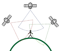
Figure 5 Determining position using a GNSS system.
Analog data transmission has traditionally used amplitude modulation or frequency/phase modulation. Digital data transmission requires far more sophisticated modulation methods to maximize error-free data transmission over the available bandwidth. Current modulation methods for the transmission of digital, discrete signals use a combination of amplitude and phase modulation, with the two degrees of freedom increasing the data transmission rate. Examples of this are amplitude phase shift keying (APSK) or quadrature amplitude modulation (QAM).
Figure 4a shows a constellation diagram for a carrier with 16-QAM modulation. The chart shows 16 different states, with each being described by a unique pair of values consisting of amplitude and a phase angle relative to the coordinate origin. In this modulation variant, phase noise causes a rotation of the entire constellation diagram, with higher values of phase noise causing a larger rotation of the points. This is seen in Figure 4b as a blurring of the exact states of Figure 4a. If this rotation is severe enough, states can be misidentified, leading to bit errors and higher bit error rates. The bit error rate can be reduced by using stable oscillators. Digital communications networks requiring the highest performance will use rubidium or cesium standards or global navigation satellite systems (GNSS)-locked OCXOs. If slightly less performance is acceptable, OCXOs with extremely low phase noise is the likely choice.
NAVIGATION APPLICATIONS
A variety of GNSS are used to determine positions on land and in the atmosphere. Well-known examples of these systems are the Global Positioning System (GPS) in the U.S. and the Galileo system in the E.U. Both systems are available for military and civilian use, although the civilian systems have lower accuracy.
The position is determined by measuring the signal propagation time of a high frequency signal from the satellites to the corresponding receiver. Comparing the transit time differences from at least three satellites allows the exact horizontal position to be calculated. Velocity data is calculated from the frequency shift caused by the Doppler effect of the satellite moving relative to the receiver. This technique requires extremely accurate clocks in the satellites and the GNSS receivers for precise time/frequency measurement. In the satellites, this is realized via cesium/rubidium atomic clocks (GPS) or via hydrogen maser clocks (Galileo), which are regularly calibrated via ground stations distributed worldwide.
Portable GNSS receivers must also incorporate extremely accurate clocks with excellent short-term stability/phase noise. If the receiver clock matches the reference clocks of the satellites exactly, the position can be determined with only three satellite signals. This concept is shown in Figure 5. In practice, the data from at least four satellites are required to compensate for the time offset caused by the poor long-term stability of the receiver clocks.
The resolution accuracy of a GNSS receiver is directly related to the noise performance of its internal time reference. Portable receivers for the mass market usually contain only simple XOs or TCXOs for generating the reference frequency, which can result in resolution accuracies in the range of several tens of meters. Professional GNSS receivers work with highly stable OCXOs, which can reduce the error in determining the position to a few centimeters due to the high short-term stability of these OCXOs.
RADAR TECHNOLOGY APPLICATIONS
Depending on the particular area of application, signals with frequencies up to 300 GHz are required for location and speed determination using radar technology. In current systems, the signal is generated by a voltage-controlled oscillator (VCO), which usually has poor frequency stability. To stabilize the signal, the VCO is connected to an extremely stable reference oscillator via a phase-locked loop (PLL). The overall performance of the system, especially the phase noise, is largely determined by the selection of the reference oscillator. In this case, the preference is to design this oscillator as an ultra-low phase noise OCXO.
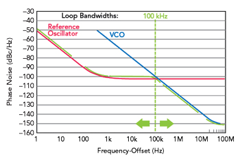
Figure 6 Phase noise improvement using a reference oscillator. Source: Revised with permission from Rohde & Schwarz.
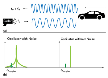
Figure 7 (a) A radar signal experiences a frequency shift from a moving object. (b) A noisy carrier signal can mask the Doppler-shifted reflected signal.
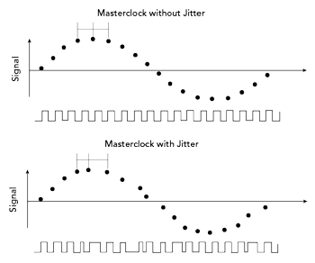
Figure 8 Effects of master clock jitter on signal sampling.
Using a PLL ensures that the phase noise close to the carrier is determined by the noise of the reference oscillator. Above a certain frequency offset, which is determined by the loop bandwidth of the PLL, the phase noise of the high frequency oscillator dominates. This effect is shown in Figure 6, where up to an offset frequency of 100 kHz the phase noise is significantly reduced by the use of the reference oscillator, compared to the free-running VCO.
Using the Doppler effect, radar technology can determine the velocity of a moving object from the frequency shift. In a simplified model of a CW radar, a signal of fixed frequency is emitted in the direction of the object to be measured. The electromagnetic wave is reflected by the measured object and travels back to the receiver of the radar unit. Depending on the target’s motion relative to the receiver, the frequency of the received signal changes. Figure 7a shows the basic Doppler effect concept.
An issue arises if the resulting frequency difference is so small at low velocities that it cannot be measured relative to a noisy carrier frequency as shown in Figure 7b. A frequency source with lower phase noise allows for a more accurate velocity determination. For a radar source with a carrier frequency of 1 GHz, an object moving at a speed of 1 km/h produces a Doppler shift of about 1.9 Hz.
AUDIO PROCESSING APPLICATIONS
Sound is a time-dependent, analog mixture of acoustic waves of different frequencies. Audio signals are degraded during analog processing because of noise in components like cables or analog amplifiers. Digital processing of audio signals overcomes some of these limitations. In this process, the analog signal is converted to a digital signal by an analog-to-digital converter (ADC) before it is digitally processed and converted back to an analog signal by a digital-to-analog converter (DAC). After this conversion, the analog signal is routed to an audio source, like a loudspeaker.
The conversion to the digital audio signal in the ADC takes place at a digital clock rate called the sample frequency fS, which is usually 44.1 or 48 kHz. According to the Nyquist theorem, these sample frequencies are suitable for digitizing analog signals up to 22.05 or 24 kHz. The sample frequency is usually provided by an internal oscillator called the master clock, which typically oscillates at a multiple of the sample frequency.
The challenge in digitization, especially in the playback of audio signals, is to use a master clock that is as accurate as possible with the lowest possible phase noise. Figure 8 illustrates the problem of a noisy master clock. During digitization, an accurate master clock ensures exactly equidistant sampling of the analog signal in the ADC, which ensures a faithful reproduction of the input signal at the output. If the master clock is not exactly periodic, this jitter influences the signal sampling. When the sampled signal is converted in the DAC, the result is a distorted output signal that does not faithfully reproduce the input signal and this affects the sound quality at the output.
Low-cost consumer products tend to use low-cost oscillators as the master clock. These oscillators typically have high values for jitter and the sound quality suffers. Professional high performance playback devices for digitally recorded music rely on crystal oscillators with extremely low phase noise to perfect the sound experience in conjunction with high-quality amplifiers and speaker systems.
CONCLUSION
High precision frequency sources, such as quartz oscillators with extremely low noise characteristics have become the undisputed standard for electronics in the 21st century. Measurement, data transmission, navigation and audio applications all place the highest demands on the signal sources. While all these applications rely on high performance signal sources, the most important parameters may be different. In telecommunications, the jitter value is important because it can be used to derive the bit error rate during data transmission. In metrology, phase noise is important with oscillators often characterized by a phase noise curve. Depending on the application, near-carrier or far-carrier phase noise may be more relevant, so phase noise values are specified at different distances from the carrier signal. Navigation applications benefit greatly from extremely stable reference clocks. If uncontrolled deviations in the time reference occur at the GNSS receiver, the accuracy of the position determination can deteriorate by one to two orders of magnitude. These and other examples show the importance of highly stable oscillators in a wide variety of applications.