
SHORT-TERM STABILITY
Along with phase noise and jitter, short-term stability can be used to describe phase deviations of a signal. The Allan deviation, named after the physicist D.W. Allan, is used as a common measure of short-term stability. The Allan deviation (ADEV) is defined as the square root of the Allan variance σ2 (τ):
Here, the Allan variance itself is defined as half of the expected value of the difference squares of two consecutive measured values (denoted here as yn and yn+1) of the normalized frequency deviation in the time interval τ. It should be noted that the ADEV is a function of the averaging time τ, which defines the period in which the average of the expected value is calculated.
Compared to the classical variance, where the deviation from the mean is measured in each case, the Allan variance only considers the deviation of two successive measured values. This leads to a convergence for all kinds of noise even with long averaging times with a mean value drift (e.g., random walk processes).
The measurement of short-term stability in the form of the ADEV can be carried out in different ways. For low frequency signals and low short-term stability, the frequency deviation between two successive oscillation periods can be determined directly by an absolute time measurement. In the following, one of many possible measurement methods is presented, which is also suitable for the measurement of high precision signals.
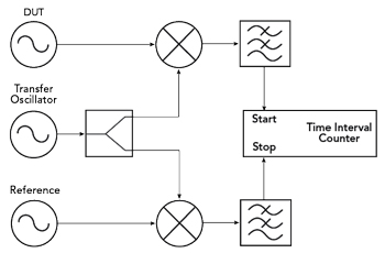
Figure 6 Determining the short-term stability using a dual mixed signal.
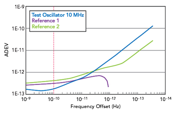
Figure 7 ADEV measurement of a 10 MHz ultra-low phase noise oscillator.
As shown in Figure 6, the dual mixer time difference method requires a reference oscillator and a so-called transfer oscillator in addition to the DUT. In this simple example, the reference oscillator must have better short-term stability than the DUT. During the measurement the transfer oscillator is slightly detuned against the other two signal sources. Here, a detuning of a few Hz up to a few kHz gives the best results, depending on the application.
By mixing this signal with the two signals of the DUT and the reference and subsequent lowpass filtering, two low frequency signals are produced. These signals are used as start and stop triggers for a time interval counter. With the interval counter the time difference between the zero crossings of both signals is measured. Depending on the desired averaging time τ, an adequate frequency offset of the transfer oscillator must be set.
If the short-term stability of the reference oscillator is not significantly better than that of the DUT, this can no longer be neglected. This effect can be mathematically corrected by using another reference oscillator. For this purpose, we refer to the so-called “three-cornered hat method.”2
Figure 7 is an example of an ADEV measurement of an ultra-low phase noise oscillator from KVG Quartz Crystal Technology with a carrier frequency of 10 MHz. Because the DUT has very good short-term stability, the measurement was performed using the three-cornered-hat method. Two oscillators with 10 MHz each were used as references. The total measurement duration was 4 hours, the sample interval was 0.1 s. The test oscillator achieved an ADEV of 1.8 × 10⁻¹³ at a time interval of τ=1 s.
RELATIONSHIP OF THE DIFFERENT REPRESENTATION TYPES
Phase Noise and Jitter
As previously described, phase noise and jitter are two different ways of describing the same physical signal property; therefore, it is obvious to look for possibilities to relate them. Jitter within a defined frequency range can be calculated from the measured values of phase noise by integrating L(f) over the frequency. The jitter power P in the frequency interval f1 to f2 is defined for a given single-sideband phase noise L(f) as:
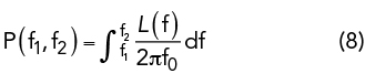
It should be noted that the phase noise is normalized by a factor of 2πf0, where f0 represents the carrier frequency. This also ensures the correct conversion of units.
The RMS value of jitter ΔT(Δf) in the specified frequency range can be calculated as the square root of the jitter power P:
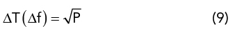
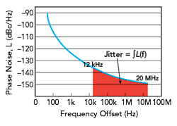
Figure 8 Jitter can be calculated by integrating the phase noise over a frequency interval.3,4
As previously mentioned, this conversion provides another indirect way of measuring jitter. Often in practice, phase noise is determined for a typical offset range from 1 Hz to about 10 MHz. From this, the resulting jitter value can then be flexibly calculated by integration over different frequency ranges (see Figure 8).
A reverse calculation of phase noise from measured values of jitter over certain bandwidths is mathematically not possible, since for this the jitter would have to be known for all possible bandwidths/frequency intervals.
Phase Noise and Short-Term Stability
Short-term stability can also be determined mathematically from the values of L(f). The transition from phase noise, which is a function of frequency, to ADEV, which is a function of time, can be described by means of a Fourier transform. The derivation of this transform is far beyond the scope of this article, so reference is made to Barnes et al.5
As a result, the Allan variance  can be written as an integral over the entire frequency range with carrier frequency f0, averaging time τ and frequency offset f as integration variables.
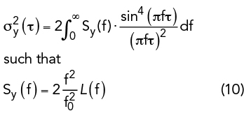
The property from Equation (10) imposes certain conditions on the spectral distribution of the phase noise, for example, that the magnitude of the phase noise becomes very small for large distances from the carrier. These constraints also go very deep mathematically, so no further consideration is given.
SUMMARY
The need for high precision frequency sources, such as quartz oscillators, with extremely low noise characteristics is undisputed for modern technology of the 21st century. Whether it be measurement technology, data transmission or navigation—in all areas there are applications that place the highest demands on signal sources.
Depending on the field of application, a different one of the described measurement quantities is proven to be practical. In telecommunications, the specification of a maximum jitter value is usually resorted to, since it can be used to derive how high the bit error rate is during the transmission of discrete information. In metrology, on the other hand, the oscillator is often characterized by a phase noise curve, in which the phase noise values are specified at different distances from the carrier signal depending on whether phase noise close to or far from the carrier is relevant for the specific application.
Since all approaches are based on the same physical phenomenon, a conversion from one form of representation to the other can be performed if the data basis is sufficiently complete.
References
- E. Rubiola, Phase Noise and Frequency Stability in Oscillators, Cambridge University Press, 2009.
- F. Vernotte, M. Addouche, M. Delporte and M. Brunet, “The Three Cornered Hat Method: An Attempt to Identify Some Clock Correlations,” Proceedings of the IEEE International Frequency Control Symposium and Exposition, August 2004.
- “Understanding Jitter Units,” Renesas Electronics Corporation, Application Note AN-815, Rev. A, March 2014, Web: https://www.renesas.com/eu/en/document/apn/815-understanding-jitter-units?language=en.
- D. Herres, “Measuring Oscillator Jitter,” EE World, August 2017, Web: https://www.testandmeasurementtips.com/measuring-oscillator-jitter/.
- J. A. Barnes, A. R. Chi, L. S. Cutler, D. J. Healey, D. B. Leeson, T. E. McGunigal, J. A. Mullen, W. L. Smith, R. L. Sydnor, R. F. C. Vessot and G. M. R. Winkler, “Characterization of Frequency Stability,” IEEE Transactions on Instrumentation and Measurement, Vol. IM-20, No. 2, May 1971, pp. 105–120.