

SMITH CHART FUNDAMENTALS
The center of the Smith chart is normalized to the characteristic impedance of the system. In the case of most RF systems, this is 50 Ω.8 All the points on the Smith chart are complex impedances that are represented by a real and imaginary part given by Equation 1:

Where:
Z = complex impedance
R = real or resistive component, which is independent of frequency
X = imaginary or reactive component
j = imaginary unit of √-1
X, the reactive portion of the complex impedance, is frequency dependent and can be described by Equation 2:

Where:
XL = inductor impedance = 2πFL
XC = capacitor impedance = 1/2πFC
F = Frequency (Hz)
L = inductance (Henries)
C = capacitance (Farads)
With that brief refresher, the Smith chart is a valuable analysis tool. It is helpful because it incorporates the effects of the total impedance in the system analysis. This is especially true of the reactive properties and will become clearer in the results section of this article.
VALIDATION EXAMPLES
Test Setup
Figure 6 Automated test stand block diagram.
The rest of this article presents the measurement and validation method using two examples. Two different test setups were used to evaluate the known-good TR module. The first setup used cables that were less than 1.5 ft. long and suspected of being faulty; they interfaced between the PNA and TR module. One PNA port was connected to the TR module input, with the output connected to the second PNA port.
The second test setup, shown functionally in Figure 6, measured the same known-good TR module with a significantly more complex configuration using an automated test station. The test station of Figure 6 uses approximately 4 ft. of cable with two more transitional connection points than the lab design validation testing setup described earlier. This test station contains a switch tree, a box containing multiple electrically actuated RF switches and an interface panel that connects short, smaller-diameter RF cables to longer, larger-diameter RF cables. These longer, larger-diameter cables transition to the faulty RF cables.
Since the goal is to ensure measurement validation with network analyzer calibration, it is important to use best practices. This means using calibrated torque wrenches, proper connector collar rotation procedures and an electronic calibration (ECAL) standard. There are many calibration standards. However, the ECAL standard, with a set of five internal reference impedances, enables sufficient testing speed and accuracy for baseline reference accuracy.9 A known-good reference cable was used to ensure measurement accuracy, stability and repeatability.
DATA RESULTS
Plotting the PNA Data
1. Capture the data or load it onto the PNA-X as shown in Figure 7
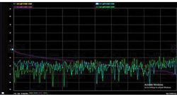
Figure 7 PNA-X data display.
2. Hover over the trace to be displayed on a Smith chart. This is the S11 trace in Figure 7
3. Right-click the trace identifier and scroll to “Format/Smith chart”
4. Left click “Smith chart”
5. This overlays the S11 trace onto a Smith chart as shown in Figure 8.
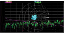
Figure 8 Smith chart data overlay.
Smith Chart Plot With MATLAB
1. Type “ver” in the command line of MATLAB and verify that RF Toolbox is installed, as shown in Figure 9
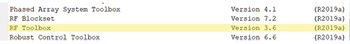
Figure 9 Display of MATLAB packages.
2. Create a new MATLAB project folder as shown in Figure 10
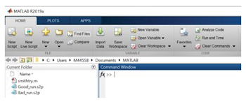
Figure 10 MATLAB environment.
3. Load the .s2p files to analyze into this folder
4. Create a new MATLAB script using the code shown in Figure 11.
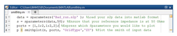
Figure 11 MATLAB code.
Running this script should return a plot like Figure 12. To magnify the display in MATLAB, click the center of the plot and scroll the mouse wheel while holding the Ctrl key.
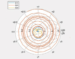
Figure 12 Smith chart data display.