

High production throughput is required in RF test facilities to meet transmit-receive (TR) module delivery schedules. Unfortunately, unexpected failures occur and determining whether the TR module, the test station, the fixture or the cables are at fault is challenging for technicians and engineers to ascertain promptly. Additionally, management is understandably impatient, trying to contain schedule creep, costs and any potential reputation damage resulting from late deliveries. Typically, the primary test failure concern relates to the design of the TR module and initial test failure investigations focus on any inherent design flaws in the TR module. These investigations must also consider whether there are more significant production and/or manufacturing producibility issues. If there are, these findings may then dovetail into concerns about personnel training, material or process planning instructions. The need to quickly isolate the failure and discover its root cause creates a crucial organizational challenge.
This type of problem necessitates a quick triage solution. This article will describe a process that uses fundamental physics of failure troubleshooting methods with Smith charts, polar charts, network analyzers and deriving and applying NASA-developed troubleshooting techniques. Using these techniques, the article will demonstrate how to quickly and qualitatively determine whether the issue lies with the module or the test station and identify the failure mechanism.1 In the examples that will be used, the enemy of the analysis was determined to be time. The goal was to develop a method that avoids lengthy, drawn-out quantitative analysis, which typically involves RF plotting and potentially, multiple retests of TR modules to determine the condition of a suspect TR module. While this legacy approach is sound, it often yields ambiguous and time-consuming results. The technique that has been developed has the triage goals of enabling the failure to be identified qualitatively, quickly and intuitively. The article will present two evidentiary examples to illustrate this method.
LITERATURE REVIEW
Earlier Research
To develop faster methods of troubleshooting, a NASA-authored paper1 offers intriguing insights. This paper incorporates an analog component current versus voltage curve tracing method. In addition, it includes a method of troubleshooting through complex impedance characterization of RF transitions, utilizing polar plots or Smith charts.2 Complex impedance characterizations made with Smith charts and polar plots of a golden, known-good and a suspect transition reveal qualitative differences; at interest is the qualitative content.
Findings and Unanswered Questions

Figure 1 S-parameter definitions for a two-port network.
In most test environments, programmable network analyzers (PNAs) do not employ Smith chart plots in the test sequence. At this point, it is worth noting that a PNA can directly plot a Smith chart or one can be post-processed in MATLAB using a .s2p Touchstone file.3 Typically, test environments limit RF PNA plots to two-port S-parameters of an AESA TR module. These are S11 and S22 (input and output return loss), S12 and S21 (reverse and forward transmission). Although pejorative artifacts can be found in suspect cables by S-parameter analysis, using this method is not as quick, does not contain as much information and is typically more cumbersome than other methods of reactance artifact discovery.
The S12 term relates to insertion loss, which is directly related to the cable’s internal center conductor. The S11 term relates to the input impedance or the relationship between the center conductor and the cable’s metallized outer shield. The S-parameter definitions for a two-port network are shown in Figure 1.
Where:
S11 = b1/a1 = forward reflection coefficient
S12 = b1/a2 = reverse transmission coefficient
S21 = b2/a1 = forward transmission coefficient
S22 = b2/a2 = reverse reflection coefficient
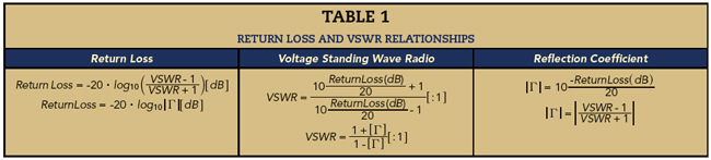
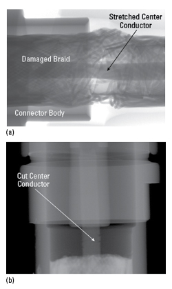
Figure 2 (a) Radiograph of damaged braid and stretched conductor. (b) Radiograph showing Teflon and center conductor cut.
Return loss is related to the reflection coefficient, Γ, and the VSWR as shown in Table 1.4
PRELIMINARY S-PARAMETER AND SMITH CHART WORK
The observation of minor reactance artifacts during slight flexion of the RF cable prompted this investigation. This bending resulted in an instability that manifested in the S11 plots. A visit to the RF cable manufacturer, along with electrical results and radiographs, confirmed that a technician used a scalpel to remove the outer cable jacket, inadvertently penetrating the outer cable shield and cutting the polytetrafluoroethylene (PTFE) dielectric that surrounds the center conductor. At higher frequencies, skin effect dominates and the signal will concentrate near the surface of a conductor. Any tears in the outer metallized braid can cause unwanted reflections that will degrade the reflection coefficient presented to the incoming signal.5 Figure 2a shows a radiograph of the damaged braid and stretched center conductor resulting from the inadvertent penetration of the outer braid and cutting of the TeflonTM (PTFE). Figure 2b shows the cut to the PTFE dielectric around the center conductor. The ideal method for removing the outer jacket involves an intentionally dull thermal stripper. With gentle pressure, there is no damage to the metallized braid or the underlying layer of PTFE dielectric.
Since S11 is most closely linked to return loss and VSWR, it is the most likely indicator of a cable assembly issue. S22 measures the reverse reflection coefficient and this measurement also showed perturbation artifacts. There was evidence of reactance effects in the S12 and S21 results with minor ripple indications in the signal content, but these ripples were on the order of tenths of a dB.5
METHODOLOGY
Methodology and Analysis
Although cable issues were detected and identified, this process was time-consuming. A quicker way to determine the problem would have been to use complex impedances, polar plots or Smith charts. Figure 3a shows reflection plots measured at Pin 1 of a known-good amplifier compared to a faulty amplifier. Below the Cartesian plots are polar plots of the same measurements. The Cartesian plots show little difference between the two amplifiers, but the complex impedance characteristics in the polar charts show a frequency shift and a more discernible difference in the response. Figure 3b shows the same analysis at Pin 2 of the amplifiers.1,7

Figure 3 (a) Cartesian and polar plot reflection response at amplifier Pin 1. (b) Cartesian and polar plot reflection response at amplifier Pin 2.
Figure 4a shows the same analysis for a good versus a faulty capacitor. While the Cartesian plot shows a slight difference at lower frequencies, the difference in the trace characteristics on the polar plot is more noticeable. Figure 4b shows this same analysis at Pin 2 and even using the polar plots, the change is very subtle.1,6
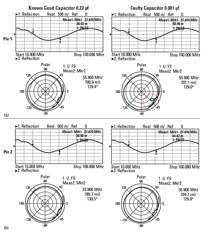
Figure 4 (a) Cartesian and polar plot response at capacitor Pin 1. (b) Cartesian and polar plot response at capacitor Pin 2.
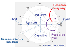
Figure 5 Simplified Smith chart.2
The thesis for the NASA paper1 is that analysis is faster using polar plots than Smith charts. They attribute this to the Smith chart’s complexity. While this belief holds some truth, many of the Smith chart complexities can be overcome with some explanation. Figure 5 shows a simplified Smith chart with the pertinent regions and formulas identified for reference.2