

Polar Plot Chart Using MATLAB
- Verify that RF Toolbox is installed as before and load the desired .s2p files into an existing or newly created MATLAB project folder
- Create the MATLAB script shown in Figure 13.
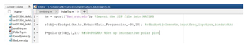
Figure 13 MATLAB polar chart script.
Running this script should return a plot like that shown in Figure 14.
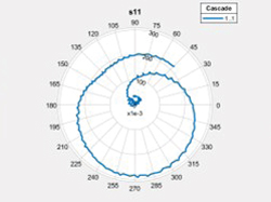
Figure 14 Polar chart of results.
ANALYSIS OF RESULTS
Example 1
The first example of these methods uses both test setups described earlier to measure the TR module. The simplified test setup uses directly connected cables with as few adaptors as possible. The more complex test setup incorporates several switch paths, more adapters and longer RF cables to the TR module. Figure 15 shows the data from both test setups plotted on a Smith chart. The data from the simplified test setup, on the left, is smooth and a bit more tightly grouped around the center of the Smith chart. The data from the automated test setup on the right shows more ripple and curling, indicative of reactive oscillations and resonances.

Figure 15 S11 data using the simplified (left) and automated (right) test setups.
Example 2
RF compression failures became an ongoing issue in actual TR module production testing. The result was that approximately 80 TR modules failed to meet the 1 dB compression requirements and were awaiting rework to replace the RFIC amplifiers. The alternative solution was determining if a test station issue was the root cause of the failures. Compounding the issue, the known-good module had been tested with a bad cable. Once modules that had previously tested good began returning for retest, evidence began pointing to the automated test station as the source of the problem.
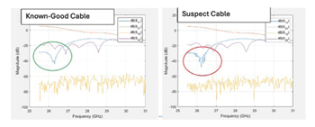
Figure 16 S-parameter plots.
With evidence pointing to a faulty test stand, the question became, were the module test fixtures, cables or switches to blame? Figure 16 shows the S-parameter measurements for the known-good and suspect cables. While the circled areas in Figure 17 show some differences, the changes in magnitude do not clearly indicate a failure.
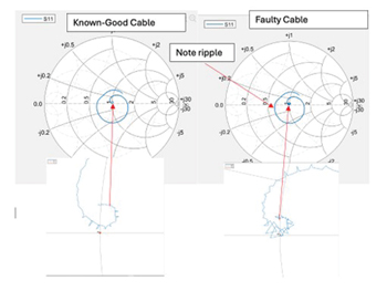
Figure 17 Smith chart plots for a known-good (left) and a faulty (right) cable.
However, the fault becomes readily apparent when the data is plotted on a Smith chart, as shown in Figure 17. The plots in Figure 16 did not indicate the reactance and oscillatory behavior shown in Figure 17. This oscillatory behavior presents as the triangular patterns that appear when the area around the center of the Smith chart is blown up for the faulty cable data shown on the right side of Figure 17. In the expanded portion of the curve, the triangular traces move from the capacitive region below the R = 0 horizontal axis to the inductive region above the R = 0 axis, which shows a resonance at these frequency points.
CONCLUSION
This effort was motivated by the need to develop a fast and efficient way to analyze and validate test stations and procedures used to measure production quantities of TR modules. This article presents a quick triage method of analyzing measurement data by plotting it on a Smith chart. With AI and machine learning (ML) techniques becoming increasingly prevalent, the attractiveness of using techniques like these to locate device failures quickly will increase. Tools like a trained MATLAB/Python ML/AI algorithm script could compare measured to saved Smith chart data.
While this is feasible, issues remain with programmability. Techniques must be developed to determine and size the appropriate boundaries to maximize the ability to find true failures and minimize the likelihood that good units are incorrectly identified as failures. Testing yields and production module throughput will increase when reasonable solutions are found for these challenges. This will positively impact rework costs and manufacturing timelines, making the business case for these activities even more attractive.
References
- R. Oeftering, P. Wade and A. Izadnegahdar, “Component-Level Electronic-Assembly Repair (CLEAR) Spacecraft Circuit Diagnostics by Analog and Complex Signature Analysis,“ NASA/TM-2011-21-216952, CLEAR–RPT–003, NASA, January 2011.
- K. Blattenberger, (n.d.), “Impedance and Admittance Formulas for RLC Combinations,” RF CAFE, rfcafe.com/references/electrical/impedance-admittance-formulas-rlc.htm.
- “rfplot.plot S-parameter data,” Mathworks, MATLAB, 2024, mathworks.com/help/rf/ref/rfplot.html.
- K. Blattenberger, (n.d.), “VSWR-Return Loss- Γ Conversions,” RF CAFE, rfcafe.com/references/electrical/vswr.htm.
- K. Blattenberger, (n.d.), “Skin Depth (a.k.a. Skin Effect) as a function of Frequency, Permeability, & Conductivity,” RF CAFE, rfcafe.com/references/electrical/skin-depth.htm.
- K. Blattenberger and J. L. Cahak, (n.d.), “Computing with Scattering Parameters,” RF CAFE, rfcafe.com/references/articles/Joe-Cahak/Computing-Scattering-Parameters.htm.
- “Impedance Matching and Smith Chart Impedance” Analog Devices, July 2022, analog.com/en/resources/technical-articles/impedance-matching-and-smith-chart-impedance-maxim-integrated.html.
- S. Bramble, “Radio Frequency (RF) Impedance Matching: Calculations and Simulations,” Analog Devices, October 2021, analog.com/en/resources/technical-articles/radio-frequency-impedance-matching-calculations-and-simulations.html.
- “Using ECAL,” (n.d.), Keysight, helpfiles.keysight.com/csg/N52xxA/S3_Cals/Using_ECal.htm.
FOR FURTHER READING
- “Automatic Fixture Removal (AFR),” (n.d.), Keysight, helpfiles.keysight.com/csg/e5080b/S3_Cals/Auto_Fixture_Removal.htm.
- E. Pedrosa, ”The Relevance of Phase Stability over Temperature in Microwave Cables, “Huber+Suhner, EverythingRF, August 2019, everythingrf.com/community/the-relevance-of-phase-stability-over-temperature-in-microwave-cables.
- Chaniotakis and Cory, “Frequency Response: Resonance, Bandwidth, Q factor,” MIT, 2006, ocw.mit.edu/courses/6-071j-introduction-to-electronics-signals-and-measurement-spring-2006/5bcec4bfba5f2e99754b77509e9e7ab4_resonance_qfactr.pdf.
- “Pulsed Measurements Using Narrowband Detection and a Standard PNA Series Network Analyzer,“ Keysight, January 2017, keysight.com/us/en/assets/7018-01160/application-notes/5988-9480.pdf.
- “smithplot. plot measurement data on a Smith Chart,” Mathworks, MATLAB, 2024, mathworks.com/help/rf/ref/smithplot.html.