
 Research and development engineers working in aerospace and defense continually strive to extend the boundaries of what is technically possible and this extends to the specialized field of electromagnetic simulation technology. One branch in this community deals with the optimization of radar cross sections (RCS), while another concentrates on the influence of the surroundings (an airplane body on the performance of communication or radar antennas, for example).
What both of these application areas have in common is the size of the electrical problem, which can typically run to many hundreds of wavelengths, and that the relevant structures are mainly surfaces and free space.
Tackling these problems is quite simply not feasible using standard volume discretization methods. CST has addressed these problem classes with the introduction of the Integral Equation solver (I-solver) for its CST MICROWAVE STUDIO® (CST MWS). It enables the user to perform accurate 3D full-wave analysis of electrically large structures, which is particularly useful in military microwave applications.
The I-solver is seamlessly integrated in the CST DESIGN ENVIRONMENT™ (CST DE). Engineers can take advantage of this easy to use interface and the sophisticated imports from a large variety of CAD formats to set up the models. The selection of the right solver is then just a mouse-click away.
The I-solver features a Method of Moments (MoM) discretization using a surface integral formulation of the electric and magnetic field integral equations. Due to the surface integral formulation the new solver uses far fewer elements than common volume methods for the described problem classes. Nevertheless, the numerical complexity of MoM is high and is not applicable to electrically large structures.
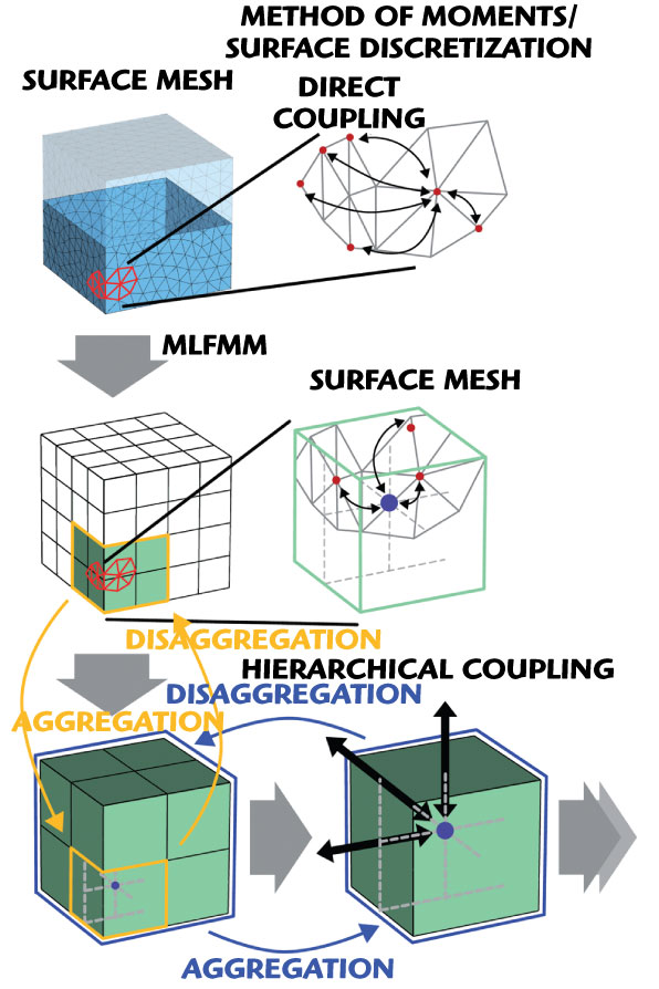
This problem is solved by applying the multi-level fast multipole method (MLFMM), as described in Figure 1. This figure shows that MoM considers the direct coupling between all elements of a mesh. In MLFMM the domain is first subdivided into separate blocks. Inside each block only the coupling to one point is considered, representing the coupling effect of the elements grouped together (aggregation). On the next level the coupling between blocks is considered. In this way a multi-level hierarchy is built-up. The coupling information is fed back through the hierarchy levels to the individual elements (disaggregation).
Now the I-solver shows numerically an efficient complexity in operations and memory for electrically large structures. One of its key strengths is the combination of higher order discretization elements with an iterative or direct solver. The higher order discretization increases accuracy compared to standard first order methods.
To reduce the numerical complexity, the built-in discretization is also capable of applying so-called mixed order discretization, where the polynomial order of the discretization function is chosen adaptively, according to the size of the mesh elements, which the automatic mesh generator chooses with respect to the structure’s features.
This means that in regions where many elements are required to resolve small details (an antenna mount, for example), a lower order discretization is used, whereas on the smooth surface of the platform or aircraft body a higher order discretization reduces the number of necessary surface elements and is ideal for military applications. An additional feature of the I-solver is the flexible MLFMM accuracy control.
It adjusts the MLFMM parameters to the individual model and, together with the powerful preconditioner, optimizes simulation time and memory requirements. However, the I-solver is not restricted to perfect electric conductor (PEC) surfaces. It can also take into account lossy metals and (lossy) dielectric materials.
The open space boundary condition best meets the demands of most antenna and RCS calculations. In addition, it features electric boundary conditions for simulating conducting grounds. The available field sources are discrete port and plane wave excitations, and waveguide ports and imported far fields will soon be available to drive simulations. The latter provides an efficient means to use the results of a high detail transient or frequency domain simulation on a large structure.
Theoretical Background
Electromagnetic field scattering by three-dimensional objects can be computed numerically using the electromagnetic field integral equations where the unknown function is the induced current distribution J(r). The integral equations can be discretized into a matrix equation system by the MoM discretization.2,3
The resulting discrete equation system is then solved by an iterative method, which usually takes N2 operations per iteration (for N unknowns). However, using a multi-level fast multipole method the numerical complexity can be reduced to Nlog(N), so that many large scale problems can be solved efficiently.2
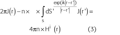
For conducting objects, the electric field integral equation (EFIE) in three space dimensions is given by
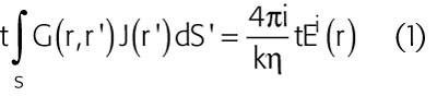
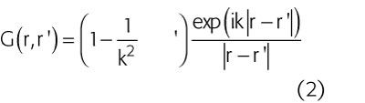
for r on the surface S, where t is any unit tangent vector on S and
For closed conducting objects, the magnetic field integral equation (MFIE) is given by
for r approaches to S from outside, where n is an outwardly directed normal.1,2 In general, either EFIE or MFIE can be used for closed conducting objects but the formulation can break down due to interior cavity resonance problems. A solution is to create the combined field integral equation (CFIE), which has numerically been proven stable for any kind of resonance effects. The CFIE for 3D-conducting objects is a convex linear combination of the EFIE and the MFIE according to

The parameter a varies from 0 to 1 and can be any value within this range. In the literature it is considered that a = 0.2 is an appropriate choice.
The MLFMM is used for solving the MoM discretization of the CFIE on a surface mesh (see Figure 1). Therefore, unlike standard MoM techniques, the I-solver reduces full coupling to one within multiple small cubic volumes of the model. These are then coupled in a similar way to a larger volume and so on recursively, until one volume remains, and scaling for numbers of cells is vastly improved at Nlog(N).
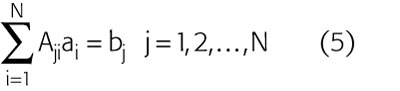
To apply the MoM to the CFIE, the unknown current J(r) is expanded using an appropriate set of N basis functions into a series according to a standard Galerkin discretization.2,3 As a result, a linear algebraic equation system is obtained, which reads
The matrix entries of A are simply given by the inner product of the selected basis functions and the integral operator of the CFIE.1 Consequently, the integral equations are approximated by matrix equations using the MoM. These linear equations can be evaluated efficiently by the fast multipole method (FMM), applying a splitting in terms representing the interactions from nearby regions.
The detailed formula is shown in Reference 1. The multilevel fast multipole method is the recursive extension of the FMM, where the matrix vector multiplication is implemented in a hierarchical or multi-level multistage fashion, which can be written as
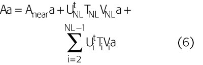
where Vi, Ti and Ui represent the matrix of aggregation, translation and disaggregation, respectively, at the ith level, and NL is the total number of levels. These matrices as well as
Anear are sparse. In the MLFMM, Vi and Ui (i < NL) are computed by interpolation and anterpolation techniques. For N unknowns, the computational complexity in memory and simulation time is the order Nlog(N).
Applications

Moving on to the applications of the I-solver, the NASA almond is a well known benchmark for RCS calculations due to its stealth properties.4 The almond is a doubly curved surface with a pointed tip (see Figure 2).
It has a low RCS when viewed in the tip angular sector. Elsewhere, a surface normal is always pointing back toward the radar, creating a bright high level specular RCS return.
In addition to specular mechanisms, surface traveling waves and creeping waves contribute to the scattering. The almond is 9.936 by 3.84 by 1.26 inches in length, width and thickness, respectively.4 Experimental data are available for a set of frequencies up to 9.92 GHz with horizontal and vertical polarizations of the plane wave excitation.

Figure 2 shows the NASA almond and displays the results of the mono-static RCS analysis for the vertical polarization at 1.19 GHz. Figure 3 shows the plot for the mono-static RCS at 7 and 9.92 GHz for horizontal and vertical polarization, respectively. The numerical results of the Integral Equation solver agree very well with the experimental data.
The simulation of a complete RCS study for a single frequency and 180° angle sweep takes less than one hour and 160 MB of memory on a PC with an Intel® Xeon™ (3 GHz) CPU.
Large Ship Simulation
The I-solver can be used to realistically simulate an antenna placement on, or radar illumination of a large transport ship, including the effects of sea water, which is modeled as a dielectric layer (see Figures 4 and 5).
The watercraft is modeled using PEC, and the dimensions are 132.8 by 20 by 20 m. The simulated monopole antenna is mounted on top of the stern.
The sea water, where the ship is embedded, is modeled as a loss free dielectric with a relative permittivity e = 80. The dimensions of the water block are 143 by 30 by 3.5 m. In total, the surface of the geometry including the ship and water covers about 77 by 77 square wavelengths at 25 MHz.
Figures 4 and 5 show the numerical results for the simulation of the full geometry at 25 MHz using a discrete port excitation for the monopole antenna.
The simulation of the antenna on the watercraft including the sea water takes less than 45 minutes and 5.2 GB memory. The simulation without the sea water takes less than one hour and 1.7 GB memory at a frequency of 150 MHz.
RCS Analysis of an Aerial Vehicle
The mono-static RCS for an aerial glider is calculated in the horizontal plane at 0.5 GHz with a 1° step size. The length of the glider and the wingspan is 14 m. Figure 6 displays the polar plot of the resulting absolute RCS value as a function of the incident plane wave direction. The total simulation time is less than 14 hours and 420 MB memory is consumed.
I-solver features a built-in function to perform such a mono-static RCS analysis fully automatically.
Conclusion
The Integral Equation solver is a specialist full-wave solver, which applies MLFMM using a MoM discretization. Its use of higher order discretizations and a flexible accuracy control, combined with a powerful preconditioner, result in outstanding performance and efficiency.
The I-solver is dedicated to the accurate 3D analysis of the electromagnetic fields in electrically large structures, and is therefore ideally suited for some problem classes of particular interest to engineers in the military microwave field.
References
1. B.M. Kolundzija and A.R. Djordjevic, Electromagnetic Modeling of Composite Metallic and Dielectric Structures, Artech House Inc., Norwood, MA, 2002.
2. D.B. Davidson, Computational Electromagnetics for RF and Microwave Engineering, Cambridge University Press, 2005.
3. A. Bossavit, Computational Electromagnetism, Academic Press Boston, Boston, MA, 1998.
4. NASA Almond, Technical Documentation, 1996, http://www.tpub.com/content/nasa1996/NASA-96-tp3569/NASA-96-tp35690015.htm.
CST of America,
Wellesley Hills, MA
(781) 416-2782,
www.cst.com.
RS No. 302