Multiple RF exciters feeding a broadband power amplifier and a broadband antenna system has become an increasingly popular form of system architecture throughout the frequency spectrum. This architecture, shown in Figure 1 , has several desirable features, the most popular of which is the reduced real estate requirement. Modern naval vessels require only one broadband HF antenna system to radiate from as many as 23 RF exciters, each carrying independent modulation. Cellular telephone base station transmitters perform similarly in the 800 MHz region, while satellite transponders depend almost entirely on this architecture in the gigahertz range.

The primary disadvantage of this architecture is the potential for interference generated by intermodulation. No other form of system architecture places multiple RF carriers in such intimate contact as those being amplified in a common power amplifier, and no matter how diligent the design engineer might be, no one has succeeded in making the high power broadband amplifier truly linear. Intermodulation products will surely be generated, but will they be detrimental?

Perhaps the most common response to that question is to simply make the broadband power amplifier as linear as possible using whatever means and then be prepared to live with the consequences. A dangerous approach, indeed, and one that raises yet another question - what are the consequences and are they acceptable?

This article intends to provide some insight into the character of intermodulation and thus help the system designer mitigate its effect. The following sections describe a means by which the harmonic output data of a power amplifier can be extrapolated to estimate the level of intermodulation products that will be caused by multiple signals of arbitrary amplitude. In addition, the effect of modulation and crest factor is considered. Armed with the frequency and an educated estimate of the level of the intermodulation products, the system designer will be better prepared to design an interference-free system.

The Amplifier Transfer Function

It is well known that the transfer function of a power amplifier can be expressed in the form of an exponential series

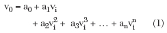
where

v₀ = output voltage
v_i = input voltage
a_n = nonlinearity coefficients of the power amplifier transfer function

In this article, only the weakly nonlinear case is of interest.¹ This assumes that the amplifier has been designed to be as linear as practical within given limits; therefore, the nonlinearity coefficients of the transfer function are quite small. In that case, a plot of the transfer function might appear as a straight line to the eye, yet there would still be enough actual curvature to generate the intermodulation products as observed by measurement.

The input voltage v_i may take the form of multiple carriers each with independent amplitude and arbitrary modulation. However, no generality is lost if, for the time being, matters are simplified by limiting the consideration in this section to sustained carriers and by deferring the impact of modulation to a later section. In this case, the input will have the form

(2)

v _i = E _A cos 2π (A)t + E _B cos 2π (B)t + EC cos 2π (C)t ...

where

E_A,E_B, = amplitudes of carriers
E_C, ... at frequencies A, B, C ...

When the input is raised to the various exponents defined in Equation 1, intermodulation products are formed. The expansion is carried out in a normal fashion and appropriate trigonometric identities similar to those listed in Table 1 are used.

When Equation 2 is substituted in Equation 1 and the expansion carried out, the result is a series of terms, each representing an intermodulation product of the general form

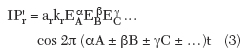
where

IP'_r = intermodulation product of order r
r = product order = α + β +γ + ...
a_r = nonlinearity coefficient of the power amplifier transfer function
k_r = trigonometric constant as given by Equation 4
E_A... = amplitudes of the individual contributing carriers
α A,β B,γ C... = type and frequency of the product

The nonlinearity coefficient from the appropriate term in the transfer function of Equation 1 is represented by a_r in Equation 3 while E_A, E_B... are as defined previously. k_r is the fractional coefficient from the trigonometric identity (1/2, 1/4... as shown in Table 1.) For convenience, these fractional coefficients are listed by intermodulation type to the fifth order in Table 2 ; however, the general mathematical expression for k_r is given by²

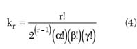
The table reveals some insight into the various types of products. For one thing, it refutes the assertion that all intermodulation products of the same order are of the same level. For example, some engineers have generalized that the third-order products may be 30 dB below the carriers, the fourth-order products -40 dB, the fifth-order -50 dB, etc. Equation 3 shows that the k factor multiplies the entire expression for the product and, in the table, the value of k varies greatly within a given product type. For example, the ratio of third-order major product (A±B±C) to the third harmonic (3A) is +16 dB. This ratio varies from as little as +6 dB in the second-order to as much as +42 dB in the fifth-order. Note also that the harmonics are a special case of intermodulation products and thus are considered accordingly. It is also interesting to note that the harmonic is the weakest product in its order.

Product Frequency, Spacing and Grouping

A transfer function term of degree r, where r is odd, will generate intermodulation products of order r plus all odd-order products less than r. For example, the cos⁷A term generates not only the frequency term 7A, but also inferior frequency terms 5A, 3A and A. Likewise, when the exponent of a transfer function is even, the term generates frequency terms of order r plus all even-order products less than r. Thus cos⁸A generates the frequency term 8A plus inferior terms 6A, 4A, 2A and a DC component.

The level of the inferior terms are generally quite small and do not often contribute significantly to the level of the total term. In many cases, the inferior terms are ignored without seriously affecting the outcome of the analysis.

Intermodulation products tend to be grouped around the fundamental and its harmonics. The higher the order and the larger the number of components, the more products there are in a group. Ultimately, the grouping from the Nth harmonic will spread to meet and overlap the groupings of the (N+1) and (N-1) harmonics. When that occurs, the entire spectrum may be filled with intermodulation products. The intermodulation product frequency and type can be anticipated from a little knowledge of how the generation process behaves.

For example, Figure 2 shows the two fundamental components to be at 5 and 6 MHz, a frequency separation of 1 MHz. Notice that the third-order (2A-B) product is at 4 MHz and the (2B-A) third-order product is at 7 MHz. Each product is spaced 1 MHz from its neighbor. This is the same spacing as that between the fundamental components. One might anticipate that the next two products in this grouping will also be spaced 1 MHz from their neighbors, falling at 3 and 8 MHz, and indeed they are - the (3A-2B) and the (3B-2A) appear at 3 and 8 MHz, respectively. In summary, the fundamentals are surrounded by odd-order products of the type (3A-B), (4A-3B), etc., and are spaced by the frequency difference of the fundamentals.

When the frequency grouping around the fundamentals expands downward beyond zero frequency, the spectrum "folds back" as though reflected from zero frequency. For example, if the frequencies A and B were 3 and 7 MHz, respectively, the spacing would be 4 MHz instead of 1 MHz. Then the (2A-B) product would be 4 MHz below frequency A, which would place it at -1 MHz. However, negative frequency appears as positive frequency so the product would appear at +1 MHz. Also, the (3A-2B) frequency will appear another 4 MHz below (2A-B), which would place it at -5 MHz. It would appear as +5 MHz. Additional products are affected similarly so the spectrum is effectively "folded back" at zero frequency.

A Prediction Formula

The harmonic output data of broadband power amplifiers is usually available from the equipment designer. Lacking that, it is not an unreasonable task to make the measurements necessary to determine the harmonic output of a power amplifier. This section develops a formula that predicts the level of a selected intermodulation product by extrapolating the measured harmonic power levels. The formula places no restrictions on the number of contributing carriers, their individual power level or the intermodulation product type. The formula will be developed first for the case of sustained carriers but will be extended later to include the effect of modulation. Equation 3 lists the general mathematical form of the intermodulation product. If a numerical value for a_r were known, then the amplitude of the product could be calculated directly since all other amplitude variables in Equation 3 are known. However, seldom is a_r known, and attempts at measuring ar are usually unsuccessful when the transfer function is only weakly nonlinear.

The factor a_r (and only a_r when the inferior products are neglected) appears in the mathematical expression for every intermodulation product of order r regardless of the intermodulation product type. Therefore, the factor a_r will not appear in the mathematical expression of the ratio of the amplitudes of any two products of order r. Moreover, if a product of known amplitude is selected to be included in the ratio, then the amplitude of the unknown product can be calculated. A harmonic of known amplitude, H_r, makes a convenient reference upon which to base that ratio.

The general expression for the r^th harmonic can be written as a special case of Equation 3

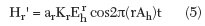
where a_r is as defined previously and K_r is the trigonometric constant associated with the harmonic of order r. E_h and A_h are the amplitude and frequency, respectively, of the fundamental that is generating the harmonic.

The amplitude ratio of the intermodulation product and the harmonic can now be written

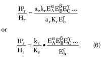
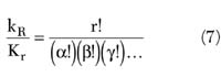
Equation 6 becomes more descriptive when Equation 4 is applied to the ratio of trigonometric constants, k_r/K_r

Substituting Equation 7 into Equation 6 and solving for IP_r results in

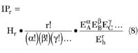
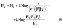
By definition IP_r and H_r can be expressed in dBw and the remaining factors converted to decibels to get

The Effect of Modulation on Intermodulation Products

For the purpose of this article, contributing carriers are divided into two categories. Sustained carriers essentially have a non-time varying amplitude. CW, FSK and PSK signals fall into this category. Time varying carriers, on the other hand, are carriers whose amplitude varies either periodically or as a random function of time. AM, SSB and multi-tone modulation are typical examples in this category.

Equation 9 shows that the intermodulation product level is a function of the product of the amplitudes of the contributing components, ... Modulation of the components can be represented by multiplying each amplitude by a unique function of time representing its particular modulation, that is,

Modulated Amplitude = [Ma_(t)EA]α

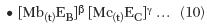
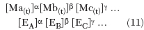
where the modulated amplitude represents the amplitude of Equation 9 when each component amplitude is modulated by individual time functions. this expression can be regrouped and written as

Modulated Amplitude =

The time functions, M_(t), vary between 1 and 0 according to the modulating information and can be a random, noise-like function characterized by a peak value, an average value and a crest factor, all of which depend upon the modulation type.

For the most part, the interference effect of a noise-like signal depends on its average value. In keeping with that concept, the time varying multiplier M_(t) can be expressed in terms of its average value by recognizing that M_(t) has been defined to have a peak value of unity. It will also have a crest factor (ratio of peak to average value) depending upon the modulation type. Therefore

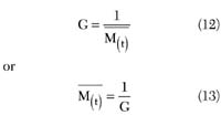
where

= average value of the time varying function
G = its crest factor as determined by the type of modulation

The crest factor for various modulation types is listed in the literature. A few are shown in Table 3 .

Equation 13 can be substituted into Equation 11 and the result converted to decibels to yield two terms which replace the third term in Equation 9 with the following result.

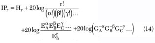
Equation 14 is near the desired form but it can be made more user friendly by converting the third term to a power ratio rather than a voltage ratio. This is done by recognizing that E = √RP and r = α +β +γ +... to obtain

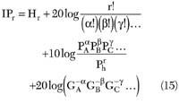
where

r = order of the intermodulation product of interest, α +β +γ +...
IP_r = predicted level of the intermodulation product of interest (dBw)
H_r = power level of the reference harmonic (dBw)
P_h = power level of the fundamental used when measuring Hr (W)
α ,β ,γ +... = exponents which describe the intermodulation product of interest
P_A,P_B, = power level of the
P_C,... contributing fundamentals (W)
G_A,G_B, = modulation crest factor of
G_C,... the contributing fundamentals expressed as a numerical ratio

Notes on Obtaining a Reference

To obtain the harmonic reference data for use in Equation 15, one would drive the broadband power amplifier to near maximum output using a single carrier. The output level of the fundamental P_h would be recorded plus the level of each harmonic H_r up to and including the highest order of interest.

It is especially important to ensure that the harmonic output of the exciter does not contaminate the harmonic reference measurements. To that end, it is highly recommended that an effective filter follow the exciter when making the harmonic reference measurements.

When higher orders are of interest, the level of the desired harmonic may not be measurable. In that case, it may be necessary to substitute the major intermodulation product type for the harmonic.

Equation 15 is limited to use of the harmonic as a reference. However, the equation can be modified to accept any intermodulation product type as the reference by following the same logic followed to develop Equation 15.³ The result is

where the primes refer to the reference parameters and the remaining nomenclature as is in Equation 15.

When using multiple fundamentals to obtain a reference, the reader must realize that many intermodulation products will be generated. It is possible that several intermodulation products may fall on a particular frequency. If the sum level of several products is inadvertently used as the reference, serious error will result.

The major intermodulation products are generated at the highest level in a particular order, so it is most desirable to use the major products if a higher level reference is needed. It is not necessary that the same type reference be used for all orders, as long as consistent parameters are entered into the formula. If a high level reference is needed, it is recommended that two fundamentals be used to obtain a second-order reference, three fundamentals be used to obtain a third-order reference, etc. Otherwise, use harmonics wherever possible.

Examples of Measured and Estimated Levels

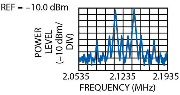
The following examples are in the HF band because HF equipment was available at the time. However, it is important to recognize that the principles involved apply to all frequency bands. Some measured product levels are shown in the spectrum analyzer display of Figure 3 .

The power amplifier yielding these data was rated at 10,000 W and its bandwidth covered the HF band from 2 to 30 MHz. The amplifier was signal loaded with four 700 W, unmodulated carriers at 2.11, 2.14, 3.5 and 3.51 MHz. However, the display shown is confined to a narrow region in the vicinity of the 2.11 and 2.14 MHz carriers to enhance detail.

A computer program calculated the product levels up to the eighth-order using the carrier powers and frequencies listed above. The harmonic references were obtained by separately driving the power amplifier to 6000 W with a single carrier at 2.0 MHz. The level of the harmonics up to the eighth were recorded in levels from -34 to -2.5 dBw using the +38 dBw fundamental. The results of the calculations are displayed in Figure 4 . In those instances where more than one product fell on a given frequency, the computer program summed the powers and reported the total.

In an attempt to gain a better understanding of how the calculated and measured levels compared, two additional 700 W carriers (at 3.53 and 3.57 MHz) were added to the drive while keeping all other conditions the same. Figure 5 shows the measured output under these conditions.

The added frequencies were chosen such that the additional intermodulation products would fall on the existing product frequencies and not further fill the spectrum. Note that almost all the product frequencies are filled to the same level. The reason for this might be attributed to the number of products that are created when the two additional carriers are added. With four carriers, only 25 intermodulation products fell within the spectrum under examination. However, with six carriers, 240 products fell within the same spectrum. Therefore, with so many products, every frequency gets an abundance of intermodulation products of varying levels such that no frequency is filled much differently from the others.

The calculated data of Figure 6 displays the same type of information as revealed in the measured data of Figure 5. The products have filled the spectrum to within -40 dB or so relative to the carriers.

Conclusion

This article provides a unique insight into the character and generation of intermodulation products in a broadband, multi-channel power amplifier. It describes a mathematical calculation that can be computerized to anticipate the effects of intermodulation in a system application.

While the agreement between calculated and measured product levels is not perfect, the agreement is indeed sufficiently favorable to make the calculations meaningful. The advance information that can be obtained from this simple work clearly justifies the effort.

References

1. Weiner and Spina, Sinusoidal Analysis and Modeling of Weakly Nonlinear Circuits , Van Nostrand Reinhold Co., New York, NY.
2. C.A.A. Wass, "A Table of Intermodulation Products," JIEE (London), Vol. 95, Part 3, 1948.
3. J.L. Smith, Intermodulation Prediction and Control , Interference Control Technologies Inc., Gainesville, VA.

J.L. Smith earned his BS degree in physics from the University of Houston and his MS degree in engineering from Southern Methodist University. He began his study of intermodulation in the mid-1950s with an assignment from Collins Radio Co. to address the intermodulation interference on the Texas Towers. These off-shore radar platforms were a part of the Air Force Early Warning Radar System located off the coast of Cape Cod. He later worked with Litton System Inc. to develop the mathematics that served as the basis for a frequency management program used aboard the LHD class Naval vessels. He is a senior member of IEEE and has authored two books, Basic Mathematics with Electronics Applications and Intermodulation Prediction and Control, plus more than 40 technical papers on related subjects. Mr. Smith is now retired and lives in Mandeville, LA.