The following sections examine these three methods for measuring amplifier linearity.

IMD OR THIRD-ORDER INTERCEPT

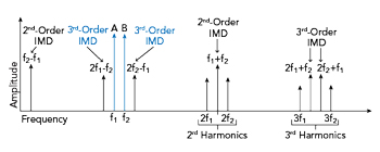
Figure 2 IMD products for equal amplitude tones A and B.

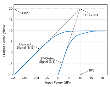
Figure 3 Calculation of TOI point (OIP3).

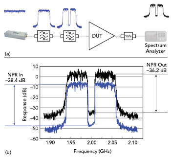
Figure 4 NPR test setup (a) and measurement (b).

When an amplifier goes into compression, it becomes nonlinear and produces signal harmonics which can mix and generate intermodulation products. The second-, third- and higher-order harmonics are usually outside of the amplifier’s bandwidth and are easy to filter. However, some of the intermodulation products are close to the intended signals and can cause IMD.

Figure 2 illustrates the intermodulation products generated from two equal amplitude tones, designated A and B. Because of their proximity to the intended signals, amplifier manufacturers are concerned with the amplitude of the third-order products and often specify a third-order intercept or IP3 value. To determine this value, the amplitude of the third-order products is plotted as shown in Figure 3. The third-order products increase at a rate of 3x the desired signal, and the intersection of the theoretical extensions of the fundamental and third-order power levels is called the third-order intercept point, denoted as TOI or IP3. The higher the IP3 value, the better the linearity and the lower the IMD. To determine the TOI, a signal generator provides the two tones, and a spectrum analyzer or vector network analyzer (VNA) measures the desired signal and third-order products.

A disadvantage of this approach is the measurement uses only two tones, while, in practice, the signal provided to the amplifier often has significantly more tones. For example, an LTE-A signal with five component carriers has 6,000 effective subcarriers or tones; a 5G NR signal may have 3,300. Two CW tones do not represent the dynamic loading that an amplifier experiences in operation. The CF is only 3 dB for a two-tone signal, yet can approach 15 dB for a 5G signal; the power supply and thermal effects would be much different with just two tones versus a high count multi-tone or noise-like signal. Another consideration is the phase coherency between tones. If the relative phase among tones is random, the measurement may be different than with phase coherent tones. This is further complicated with LTE or 5G signals, where the physical layer is based on the orthogonality of the carriers.

NPR

Another measurement for quantifying amplifier linearity is NPR. Here, white noise is used to simulate a multi-tone carrier signal. An additive white Gaussian noise generator has a high CF and represents a wideband communication signal much better than a two-tone IMD stimulus. The noise is band-limited by a filter, to either the useful bandwidth of the amplifier or the bandwidth of the expected signal. The resulting signal is passed through a notch filter with a notch typically greater than 50 dB below the passband amplitude and a width of approximately 1 percent or less of the filtered noise bandwidth (see Figure 4a).³

This signal is applied to the input of the amplifier, and the amplitude is increased to the point of nonlinearly. As discussed above, in the nonlinear region, the multiple tones mix to create intermodulation products. Because the noise signal is equivalent to many tones, the individual IMD products cannot be measured easily. Instead the aggregate power of the IMD products at the notch frequency is measured; as the products increase, the effective depth of the notch decreases. Figure 4b shows the input signal to the amplifier has a notch depth of 38.4 dB, and the depth of the notch in the amplified signal decreased to 36.2 dB, indicating the amplifier is in compression. Like two-tone IMD testing, NPR is typically measured with a spectrum analyzer or VNA. An added expense is a high quality filter with sufficient notch depth to observe the IMD products of interest.

CF

The third approach for characterizing an amplifier’s linearity is with a CF measurement. CF is the ratio of peak-to-average power. Like the NPR measurement, the amplifier input is band-limited noise to drive it with a signal approximating what an amplifier would see in actual use.

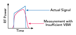
Figure 5 Incorrect peak power measurement from a sensor with insufficient bandwidth.

Using a directional coupler or signal splitter, the incident signal is measured with a wideband peak power sensor. The video bandwidth of the sensor, as well as the coupler or splitter, should be at least as wide as the bandwidth of the noise signal; otherwise, the measurement will be distorted (see Figure 5). A second measurement is made at the output of the amplifier, including any attenuation needed to keep the signal in the measurement range of the sensor, and the CFs of the input and output signals are compared. If the output CF is less, the amplifier is compressing the signal’s highest peaks. For the most accurate measurement, a third sensor can be used to determine if a portion of the input signal is reflected rather than amplified. By comparing the input and output average power, the amplifier’s gain can be determined. Figure 6 shows the test setup.

As previously noted, just monitoring gain changes with average power measurements does not give an accurate indication of amplifier linearity in operation. An average power gain reduction can be significantly smaller than the compression observed with a multi-tone signal.

BENEFITS OF CCDF

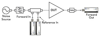
Figure 6 CF measurement setup.

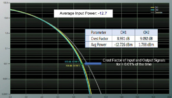
Figure 7 Amplifier CCDF for −12.7 dBm average input power.

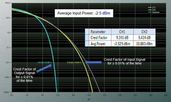
Figure 8 Amplifier CCDF for −2.5 dBm average input power.

The CCDF can provide additional insight into amplifier performance. For each power level, the CCDF curve shows the amount of time the signal spends above the average power level. Equivalently, the CCDF curve displays the probability that the signal power will be above the average power. To illustrate, Figure 7 shows the CCDFs for an amplifier with an average input power of -12.7 dBm, comparing the input (channel 1), output (channel 2) and ideal Gaussian signals. Approximately 0.01 percent of the time, the signal will have a CF of approximately 9 dB, and the input and output CFs match within 0.2 dB. When the input power is increased to -2.5 dBm, the CF at the output degrades significantly to 5.4 dB, indicating a substantial degree of compression (see Figure 8).

The additional information provided by using the CF and CCDF sheds light on the applicability of classes of amplifiers previously thought to be unacceptable for communications applications. For example, the Empower RF Systems model 2223 PA uses GaN on SiC in a class AB broadband amplifier. It has a wide frequency response from 500 MHz to 6 GHz, 53 dB gain and 150 W minimum output power. Its class AB design has very high efficiency, given its bandwidth, and is compact. This amplifier exemplifies a multi-mode amplifier, one capable of efficient “brute force” power and linear performance for communications or test applications. Traditional methods for measuring linearity will incorrectly characterize its linearity and suitability for transmitting digitally modulated waveforms.

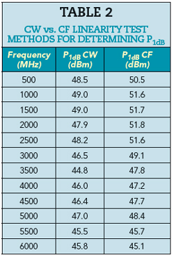
Two linearity test methods were performed on the PA to determine P_1dB. The first used a CW signal, where the input power level was increased until 1 dB compression was measured and repeated at multiple frequencies across the band. The second method used CF for determining P_1dB, with a 64 QAM signal having a CF of 6.3 dB. To determine the 1 dB compression point using CF and CCDF, at each test frequency, the input power was increased until the measured output CF decreased 1 dB to 5.3 dB. Table 2 compares the results of the two methods, showing the CW method gives a P_1dB compression point about 2 dB below the P_1dB measured with the CF method. The difference is because of transistor gain variation versus temperature. In most GaN HPAs, the gain per stage varies -0.012 dB/°C of junction temperature.

In a class AB amplifier, the transistor consumes more power as the output power increases, and as the junction temperature increases, transistor gain decreases. With a class A amplifier, one sees the opposite. For example, consider a class A amplifier with a CW input signal. When the output power is low, the transistor consumes the most power and junction temperatures are near maximum for the operating condition. As the output power increases, the junction temperature of the transistors reduces, resulting in gain expansion which extends the “apparent” compression point. However, when the same amplifier input is a modulated signal with a high CF, the device does not exhibit gain expansion since the transistor junction temperature correlates to the average power and remains high. This underscores the best practice of stimulating an amplifier with a signal representing the actual signal it will see.

Examining the theory behind this phenomenon, the output power in a linear PA can be described by the equation:

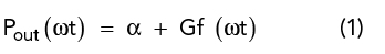
where f(ωt) is the input signal, ∝ is a constant and G is the gain of the amplifier. For a GaN amplifier, G varies with temperature as described by:

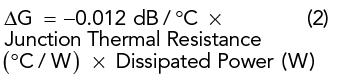
For a class AB amplifier, if the thermal resistance is 1°C/W and the power dissipation from small-signal to large-signal increases by 50 W, Equation 2 yields a gain reduction of 0.6 dB solely due to the increase in junction temperature. Conversely, when the same device operates in class A, the power dissipated decreases since a portion of the power goes into the load. Using the same gain equation, the resulting gain increases because the power dissipation is reduced. In both cases, this gain variation is not indicative of the true linearity of the PA, i.e., the linearity that changes the fidelity of the input signal. True linearity is assessed by measuring the compression of signal peaks relative to the average power.

CONCLUSION

Use of GaN technology will accelerate in the coming years, driven primarily by advances in commercial and military radar and the build-out of 5G networks. 5G has very demanding linearity requirements. Traditional tools for assessing amplifier linearity are no longer sufficient to predict real world performance. Compared to traditional tools, analyzing amplifier compression by measuring CF reduction combined with the statistical analysis offered by CCDFs provides a clearer and more accurate indication of signal compression. It is simpler, more accurate, less prone to errors and lower cost. This tool also provides insight into how amplifiers previously considered unsuitable for communications can be good alternatives to the amplifiers traditionally used.n

REFERENCES

1. A. Moore and J. Jimenez, “GaN RF Technology for Dummies®, Qorvo Special Edition,” John Wiley & Sons, Inc., 2015.
2. “RF GaN Market: Applications, Players, Technology and Substrates 2018-2023 Report,” Yole Développement, 2018.
3. A. Katz and R. Gray, “Noise Power Ratio Tutorial,” Linearizer Technology, Web: www.lintech.com/PDF/npr_wp.pdf.