GaN amplifier linearity is measured using three techniques: intermodulation distortion, noise power ratio and crest factor (CF). The CF method proves to be more relevant to actual operating conditions, while demonstrating the advantages of greater accuracy, simplicity and lower cost.

GaN devices continue to be key elements in many radar, electronic warfare, satellite and terrestrial communication systems. They offer several advantages.¹ For example, GaN has a high breakdown field due to a large bandgap that enables GaN devices to operate at higher voltages. Combined with a high saturation velocity and correspondingly large charge capability, GaN devices are ideal for high power applications. Add to this excellent thermal conductivity, and it is easy to see why applications for GaN devices continue to grow. In a recent study, Yole Développement expects the GaN industry to grow with a 23 percent compound annual growth rate between 2017 and 2023, driven by telecom and defense applications.²

Some of the most popular GaN devices are wideband RF power amplifiers (PA). Amplifiers are described by multiple characteristics including gain, frequency response or bandwidth, power output, linearity, efficiency and noise figure. Two key characteristics often used to describe the quality of an amplifier are linearity and efficiency. The relative importance of these two attributes depends on the application. For example, in a satellite-based system, efficiency may be more important, as limited power is available. In terrestrial wireless communications, the relative importance may be more balanced. Communication systems, such as those based on 5G standards, use wideband modulation with significant linearity requirements. In addition, because of the amount of base stations needed to support these systems, attention to power efficiency is required to manage operating expenses. Unfortunately, the output power levels to maintain amplifier linearity are often well below the levels needed for maximum efficiency.

MEASURING LINEARITY

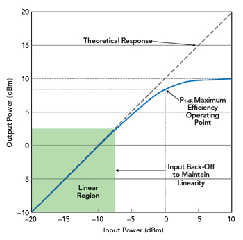
Figure 1 Typical amplifier power transfer characteristic.

This article focuses on the applications where amplifier linearity is the critical attribute. Figure 1 illustrates typical amplifier behavior. Linearity is measured by increasing input power and observing output power until the amplifier enters compression. Often, amplifier linearity is specified as the input power level where the corresponding output power is 1 dB lower than the theoretical linear response, often designated as P_1dB. Historically, this has been considered the point where amplifiers operate most efficiently.

With the simultaneous need for linearity and efficiency, it is crucial to optimize the input back-off. Too much back-off sacrifices efficiency and causes the amplifier to be oversized to reach the required output power and more expensive; too little causes increasing compression and signal degradation. Therefore, measuring amplifier linearity accurately under realistic operating conditions is important to GaN amplifier designers.

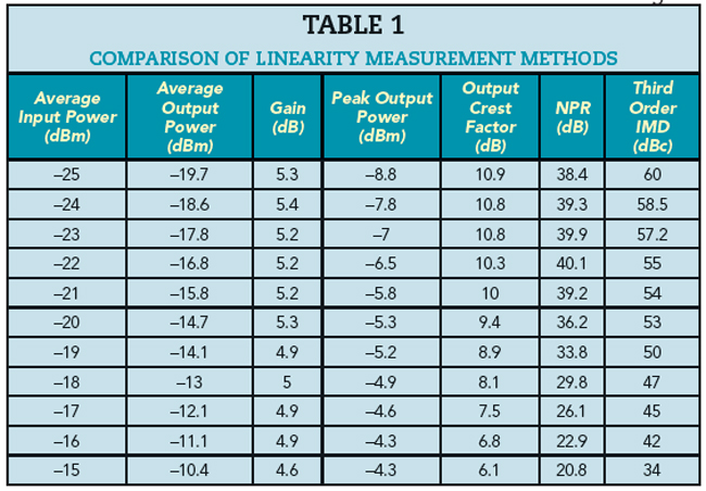
Of the ways to measure and express amplifier linearity, three common methods are: 1) intermodulation distortion (IMD), 2) noise power ratio (NPR) and 3) CF or peak-to-average power ratio. Table 1 compares measurements made with the three approaches. Using a Noisecom noise source or a two-tone source, a signal is applied to the amplifier, with the input power starting at -25 dBm and increasing in 1 dB steps until reaching -15 dBm. Reductions in gain, CF, NPR and the difference between the intermodulation products and carrier signals all indicate an amplifier is nonlinear. All three measurements show that as the input power increases, the amplifier compresses the signal and operates nonlinearly; however, only the CF method clearly reveals the amount of compression. The three measurements show the amplifier starts compressing when the average input power is approximately -20 dBm. Although the gain begins reducing at around -20 dBm, even at -15 dBm, the gain is reduced by less than 1 dB. In contrast, the other linearity measurements show more significant compression of the peak power. For example, the CF decreases by more than 3 dB.

Compression measurements only using average power are not sufficient to identify significant impairments for signals with high CFs, such as the OFDM signals used in 5G and Wi-Fi communication. Comparing the three linearity measurements shows clear advantages to the CF approach:

• Clearer indication of meaningful signal compression - Conventional, average power compression measurements do not reflect the signal impairment occurring in wideband communication signals.
• Lower cost - The CF approach uses low-cost noise sources and wideband USB peak power sensors. Test systems using spectrum analyzers can cost multiples of the price of a USB sensor, and an analog signal generator adds expense.
• Simpler, less error prone - Spectrum analyzers can be complex to configure and the results may be difficult to interpret.
• Higher accuracy - The uncertainty of a power sensor measurement is usually in the tenths of a dB, while spectrum analyzers and signal generators are typically 1 to 2 dB.

Using the complementary cumulative distribution function (CCDF) of the CF adds the probability of occurrence to the measurement. CF measurements provide a single value based on a calculation from the highest single peak power value in a population of measurement samples. However, if this peak only occurs once out of a million samples, it may not present a problem during actual use. Quantifying the degree of peak impairment using CCDF can provide the value of CF that occurs with a specific probability - 0.1 percent or one in 1,000 samples, for example - which is helpful when considering the effects of amplifier compression on bit-error-rate or error vector magnitude.