
An accurate accounting of manufacturing factors such as surface roughness and plating details are missing from the model used for EM simulation, so the in-band insertion loss will likely be higher than this initial estimate. The model approximates 80 percent of the ideal conductivity as a starting point. The quality of the silver plating is very process dependent. The measured data from the manufactured and tested filter can be used to adjust model conductivity information.
Coupling Coefficient Simulation
From the Chebyshev lowpass filter parameter values (g in Table 1) the external Q and the coupling coefficients (kij) for the resonant pairs are calculated based on Equations 3 and 4, respectively, using a 2.85 percent bandwidth.
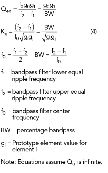
These calculated values provide the targets for the physical design. The next step is to build the coupling coefficient design curves using an EM model of the coupled resonators in order to determine the necessary spacing.
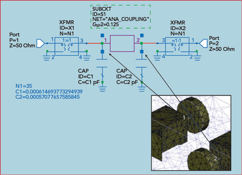
Figure 6 Ports introduced for port tuning of coupled resonators.
Two resonators based on the initial resonator study are enclosed in a metal cavity and loosely coupled to the input and output ports, as shown in Figure 6. The resonators are identical and resonate at frequency f0. The coupling between the resonators results in a displacement Δf of the resonant frequencies, which is known as the coupling bandwidth. By dividing the coupling bandwidth by the ripple bandwidth of the filter, the normalized coupling coefficient is obtained. The normalized coupling coefficient divided by the center frequency provides the Chebyshev lowpass coupling coefficient. The resonant frequency occurs at the mid-point between the two peaks, as shown in Figure 7.
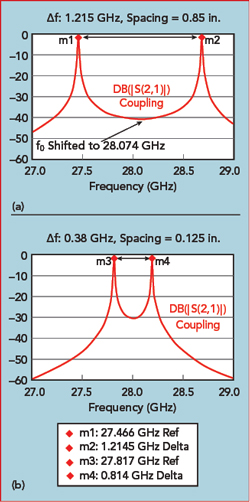
Figure 7 Simulated transmission characteristics of two resonators enclosed in a metal cavity and coupled to input and output ports: cavity spacing equals 0.085 in. (a) and 0.125 in. (b).
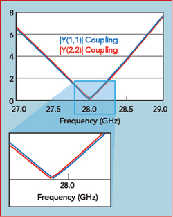
Figure 8 The f0 shift is addressed through tuning c1 and c2 values using optimization.
The more closely the resonators are spaced, the farther apart are the resonant peaks; this corresponds to higher coupling. As the resonators move farther apart the coupling gets progressively weaker and the two peaks merge together at the original resonant frequency. It can also be seen that the center frequency between the peaks in Figure 7a are shifted upward 74 MHz for the case where the resonator spacing is 85 mils. The admittance vs. frequency for these two ports is simulated and the capacitor values are optimized to zero out the admittance at 28 GHz, which re-centers the resonant frequency of the coupled pair (see Figure 8). The impact of the small amount of capacitance added or removed in order to center the coupled resonance can then be replaced by adjusting the resonator length to add/remove an equivalent amount of capacitance.
Calculating Kij Curves From Parametric EM Analysis
Dividing the normalized coupling coefficients by the 28 GHz center frequency provides the coupling coefficients that are needed to match up to the lowpass Chebyshev parameter values.
From Kij calculations:
[K1,2],[K4,5] = 0.02466
[K2,3],[K3,4] = 0.01812
Coupling bandwidth [1,2][4,5] =
690 MHz
Coupling bandwidth [2,3][3,4] =
507 MHz
(= Kij x 28GHz)
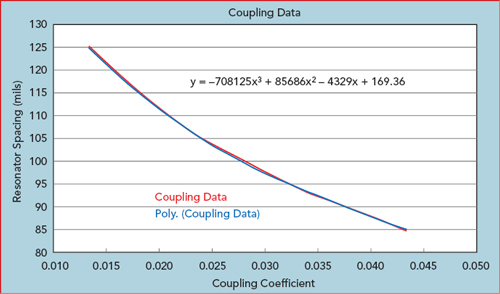
Figure 9 Inverse relationship between the amount of coupling between resonators and their spacing.
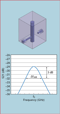
Figure 10 External coupling is found by measuring the 3 dB bandwidth of the resonance curve.
By parameterizing the spacing and tweaking the resonator length through port tuning, a curve relating coupling coefficients to very accurate resonator spacings based on EM analysis can be calculated. From this curve the spacing necessary to achieve a required coupling is determined. The curve in Figure 9 shows the anticipated inverse relationship between the amount of coupling between resonators and their spacing.
Parametric Modeling of the Tapped Resonator
The next step is to determine the physical details of the tapped resonators that provide the input/output to the filter. The external coupling is found by measuring the 3 dB bandwidth of the resonance curve denoted by Δf3dB (see Figure 10). The external Q is Qext = Qloaded = f0 / Δf3dB. It is also possible to determine the external Q by measuring the group delay of S11.
A parameterized EM model including a coax feed that taps into a single resonator is created and the distance from the bottom of the housing to the center of the coax tap is parameterized so that it can be adjusted to different heights to achieve the external Q calculated from the Chebyshev lowpass parameter. A lumped port is also placed between the resonator and tuning screw to support port tuning for addressing shifts in the resonator frequency due to the tap (see Figure 11).
EM analysis of the tapped resonator provides the time delay response as a function of frequency for different tap heights (see Figure 12). The time delay response is used to derive the external coupling. Parametric simulation enables the generation of an external Q vs. tap height curve, from which the tap height necessary for the required Qex can be directly chosen (see Figure 13).
Port Tuning
Parameterization is used to sweep values and generate the individual components that are combined to reproduce the entire filter and finalize the design through port tuning using the equal ripple optimization routine. While today’s EM simulators are quite fast and powerful, EM simulation times for low-order filters is still on the order of minutes or tens of minutes. Port tuning moves the optimization process from the EM domain to the circuit theory domain, where simulation times are much faster. Adding a port at each resonator enables rapid tuning of each resonator and the coupling between resonators (see Figure 14).
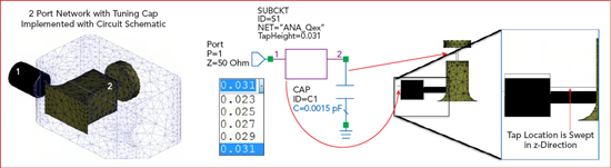
Figure 11 Single resonator EM model includes a coaxial feed with a parameterized tap feed height to adjust external Q.
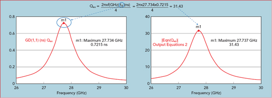
Figure 12 Simulated reflected time delay for a given tap height.
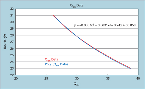
Figure 13 Qex vs. tap height based on a parameterized swept EM analysis of reflected time delay.
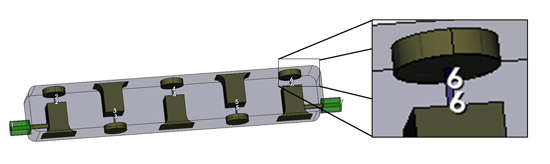
Figure 14 Adding a port at each resonator enables tuning the frequency of each resonator and the coupling between resonators.
With each resonator loaded by a 50 ohm port, the raw coupling between resonators (not coupling coefficients per se) is simulated and the S-parameter variation across the simulation domain is extremely smooth (see Figure 15). In fact, for a narrowband filter, only five to 10 discrete frequencies across the simulation domain are required for the circuit simulator to generate a smooth frequency response plot through interpolation.
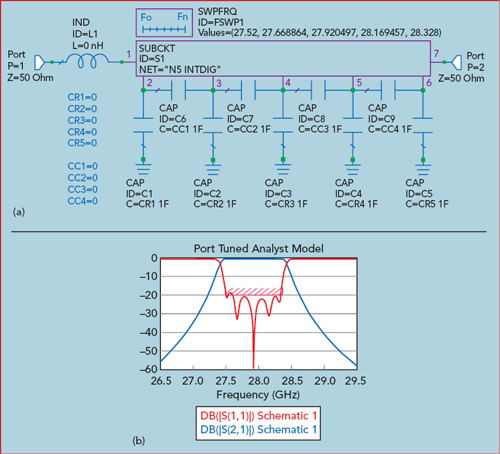
Figure 15 Coupling parameter simulation (a) and resulting S-parameters (b).
With port tuning, the resulting capacitance values reveal the tuning requirements for the 3D EM model. Both positive and negative capacitance values can be used in circuit simulation. For the resonator tuning (port to ground capacitors), a negative capacitance value indicates that the resonator (EM model) is tuned too low. Positive capacitance represents a resonator that is tuned too high. For adjusting the coupling (port to port capacitors), a positive series capacitance indicates that the coupling is too strong in the EM model (the resonators are too close).
The process is repeated until the capacitances become sufficiently small. Convergence is guaranteed if the changes are not too large. Once resonator sensitivities (kHz per mm) are known, capacitance values can be converted into physical changes of the structure. Figure 16 shows the dimensions for the final design, derived from the port tuning.
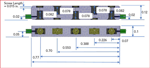
Figure 16 Final dimension of the filter design, derived from port tuning.
SIMULATED vs. MEASURED RESULTS
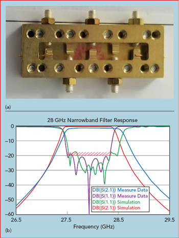
Figure 17 Pre-plated cavity (a) and simulated vs. measured results (b).
From this design, the filter manufacturer (Reactel Inc.) built and tested the cavity filter, shown without the cover in Figure 17a. The frequency response of the measured filter and simulated model is shown in Figure 17b. As designed, the target response is achieved with moderate screw tuning. More precise tuning would better replicate the optimized, simulated result.
Manufacturing Tolerances and Yield Analysis
Modern CNC machines offer 0.0002 in. tolerances, not including tooling and fixturing. The relationship between 3D EM model and port tuning capacitors (resonators and coupling) can be used to perform yield analysis using the circuit simulator, allowing physical tolerances from manufacturing process to be translated into capacitor tolerances for yield analysis. Yield analysis of microwave circuits is often done with a Monte Carlo-type analysis with a large number of iterations. Running these iterations in the EM domain is prohibitive, but if the computed sensitivities convert a capacitance to a physical dimension, yield optimization is possible through the circuit simulation.
CONCLUSION
A practical design method that is independent of filter type/construction has been demonstrated, showing a robust equal ripple filter optimization that is a fast and intuitive alternative to design by synthesis and an efficient approach for port tuning complex EM-based filter models. EM tools continue to mature and add capabilities/speed, making it practical to include them in an optimization loop. This technique has been used to address the challenge of designing highly sensitive mmWave filter designs.