
Pulse compression radar achieves processing gain by matched filtering. First described by D. O. North in 1943 at RCA Princeton Laboratories, systems can implement matched filtering for wideband radar receivers by using dispersive surface acoustic wave (SAW) devices as pulse compressors when designers are seeking large time-bandwidth products, low latency and high dynamic range. Usually the transmitter side waveform generator is also a dispersive SAW device, making an expanded pulse “the chirp.”
Modern systems can improve on this matched filter system by “matching the matched filter.” The concept is to precisely measure a particular dispersive SAW compressor using a high resolution VNA and generate an expanded pulse that is matched to that particular SAW compressor, rather than manufacturing custom compensation networks for each SAW compressor. The advantage of this strategy is improved sidelobe performance and the opportunity to compensate for system-wide errors in the transmitter.
An example system is characterized as bandwidth B = 460 MHz and an expanded pulse width T = 12.5 µs, centered at Flo = 331.8 MHz. The quadratic phase law for this linear FM (LFM) example can be expressed in normalized time tn as:
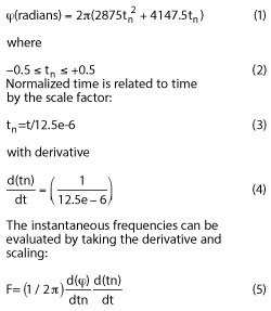
The last factor arises from the derivative chain rule.
Table 1 indicates values at the start, middle and end points. This is an up-chirp, as the frequency is rising in time, and the difference in frequency from start to end is 561.8 - 101.8 = 460 MHz, the dispersive bandwidth of the expander. A digital waveform generator can be built based on a quadratic phase accumulator cascaded with a cosine angle-to-amplitude process and a digital-to-analog converter (DAC). A suitable sampling system can be based on Fsam= 4 × 331.8 = 1327.2 MHz, yielding a Nyquist bandwidth sufficient for this example.
In practice, the phase match must be accurate to better than 0.1 degree to achieve high quality sidelobe suppression. Phase errors in wideband dispersive SAW compressors are observed to have a significant cubic error term on the order of 30 degrees peak-to-peak, in addition to small higher-order terms.
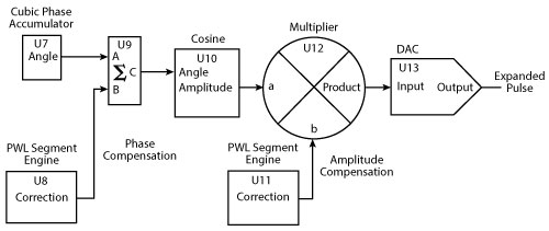
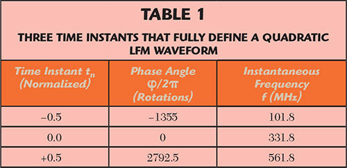
Figure 1 Digital waveform generator.
Precision Digital
Accordingly, the design has been elaborated beyond the basic approach by using a third-order polynomial for the phase law, adding a secondary phase modulator based on piece-wise linear segmentation and adding an amplitude modulator, also based on piece-wise linear segmentation. The overall organization of the digital waveform generator is shown in Figure 1. A phase domain modulator is an adder, while a multiplier is used in the amplitude domain. This generator uses a cubic phase law accumulator (U7) and modulators (U9 and U12) to modify the instantaneous phase and amplitude. The modulators are driven by piece-wise linear segment engines that correct high order imperfections. All digital processing is clocked at the rate Fsam.
Figure 2 Cubic phase accumulator.
The structure of the cubic phase accumulator is simply an extension of the quadratic form (see Figure 2). This block diagram lays out the structure of the phase accumulator (U7 in Figure 1): U1 is a two-port adder; U2 is a pipeline register, clocked at Fsam. The third-order system is a cascade of the U1, U2 structure with two additional sections (U3, U4 and U5, U6) to achieve cubic phase. The constants a, b, c and d are described below.
The polynomial form of the cubic phase law is:
As this is a sample data system, normalized discrete time is integer multiples (m) of the clock period:

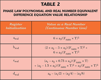
The cubic phase accumulator requires initial values loaded into the registers before the start of waveform generation. The values are partially developed in Table 2.
It might appear unnecessary to include a constant a0 in the phase law, but it proves useful in controlling the phase to exactly 270 degrees at the instant of the start of chirp. This corresponds to a rising zero-crossing of the cosine function and is readily observable on an oscilloscope. Furthermore, in the example there are 1,355 rotations from the start to the middle, so that point should also be 270 degrees modulo 360. The end point of the chirp is another 2,792.5 rotations, so that will correspond to a falling edge zero-crossing. Figure 3 illustrates the precise location of the start of the chirp waveform, which was created for this example by a definition for a0 such that the phase is 270 degrees at tn = -0.5. Note the waveform starts before tn = -0.5 to allow for edge shaping. The marker at two divisions past center indicates the rising zero crossing, where the instantaneous frequency is 101.8 MHz.
A phase accumulator could be implemented in hardware handling floating point numbers, but that would consume significant resources. Conversion by scaling and casting to integers allows for a simple accumulator, and scale factors that are powers of 2 provide for simple manipulation. For example, a 32-bit accumulator would apply a factor of 232 to each of the register initialization values. Hence the constants for Figure 2 are
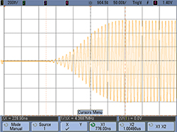
Figure 3 Chirp waveform.
The reals are cast to integer values and loaded into the accumulator at the starting instant. By meeting the Nyquist criteria, we are assured that areal, breal and creal are all less than 1. The phase angle result at U6 is produced once every period of Fsam. Removal of the 232 factor is trivial: move the (conceptual) binary point from after the LSB to before the MSB of the digital word. Figure 4 shows the error that arises when the values from Equation 1 are applied to a third-order phase accumulator with a3 set to zero. The errors are fairly small for chirp applications, considering that the chirp has 4,147.5 rotations. In fact, it seems possible to correct for that error with a subsequent phase modulator, as it is known to be exactly repeatable — but wait, it gets complicated.
A more complete error model requires understanding the contribution of a cubic term. Chebyshev polynomials are a convenient way to add a small ripple to the pure quadratic form. For example, a scaled T3() is 32 × tn3 - 6 × tn, which adds two full rotations from start to finish (720 degrees). This tiny T3() is directly added to the corresponding powers in equation 6. The same 32-bit phase accumulator produces dramatically different and poorer results (see Figure 5). Now the end point error is 11,500 degrees, which is a tall order for the subsequent phase modulator to correct. The heart of the problem is that the introduction of the cubic term has increased the rate at which error accumulates. Moving to a 48-bit accumulator looks much better (see Figure 6).
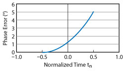
Figure 4 Phase error in a 32-bit phase accumulator with only quadratic terms.
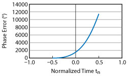
Figure 5 The 32-bit accumulator fares poorly when a cubic term is introduced.
In application, there is one more consideration: the coefficients in equation 6 are convenient for dynamic control of the phase accumulator. If small changes are needed, due to temperature variations for example, it is simple to adjust those parameters. However, by perturbing the coefficients by small amounts, additional errors become visible. A Monte Carlo analysis with the coefficients varied over a range of ±450 ppm indicates that a 52-bit phase accumulator meets the requirements. Figure 7 shows the phase error at the last sample, which is always the largest error. The worst case error does not exceed ±0.03 degrees. Operationally, this means when a small change is made to the cubic polynomial, the phase accumulator might have a change in error of twice this amount, or 0.06 degrees. The end point errors are random; they arise due to small rounding errors when the real numbers in Table 2 are cast to integers.
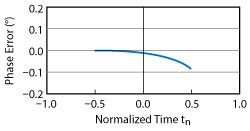
Figure 6 Reduced phase error in a 48-bit phase accumulator with a cubic term.
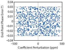
Figure 7 52-bit cubic phase accumulator error vs. coefficient variation, where B = 460 MHz, T = 12.5 µs and Fsam = 1327.2 MHz.
A worst-case bound can be calculated by assuming that the coefficient errors (eps) are all the same magnitude and the same sign at each stage of the phase accumulator. Normally the eps will be of different signs and magnitudes, and some might even be exact machine numbers. Also, some eps will cancel out the contributions of other stages. The mathematics to use for error accumulation is almost the same expression as for phase accumulation; it really is an error accumulator. Using this assumption, for n accumulations of a coefficient quantizing error eps, the total phase error is:
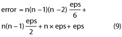
The first product term isn’t present for quadratic phase accumulators. It can be seen that the cubic phase accumulator has a large first term. Using equation 9, Figure 8 shows that for a phase accumulator of M bits, a worst-case rounding error eps = ½ (2-M) occurs at each increment and the relative position in the accumulator cascade magnifies the contribution. This provides design guidance on keeping the error less than 0.03 degrees. This example system was actually implemented at greater than 52-bit accumulator word size to allow for much larger expanded pulse durations (T). A duration of 47 µs is easily accommodated.
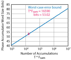
Figure 8 Accumulator field width vs. number of accumulations needed to keep the phase error less than 0.03 degrees.
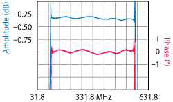
Figure 9 Demodulated amplitude and phase responses (with respect to a perfect quadratic) of the expanded pulse from the digital waveform generator.
Compensating the Expanded Pulse
A demonstration of the programmable compensation capability of the digital waveform generator is provided by observing its behavior when self-correcting. The goal of self-correcting is to generate constant amplitude and pure quadratic phase. This performance (see Figure 9) is the result of a cubic phase accumulator, piece-wise linear phase compensation of 122 segments and piece-wise linear amplitude compensation, also 122 segments. The demodulated amplitude and phase responses (with respect to a perfect quadratic) show a peak-to-peak amplitude error of 0.0875 dB and a peak-to-peak phase error of 0.375 degrees over a 460 MHz bandwidth. The expanded pulse was auto correlated, and two time spurii were seen positioned at -51 dB at 7 ns, and -57 dB at 10.56 ns. They were not paired-echo responses. The cause of these spurii was not investigated but most likely arose from return loss errors around a bandpass filter, and return loss error on the 41 inch long coaxial cable leading to a high performance oscilloscope.
The phase ripples in Figure 9 are a 90-degree shifted version of the logarithmic amplitude ripples, curiously like a Hilbert transform, and suggesting a minimum phase system. Strangely, the ratio of the amplitude ripple in dB to the phase ripple in degrees is 0.375/0.0875 = 4.28, which is better than the expected ratio for a minimum phase system of 6.6. Note that the phase accumulator and piece-wise linear phase and amplitude modulators require initial data as waveform parameters. In this example, there are 4 × 52 bits in the phase accumulator and 122 × 2 × 32 = 7,808 bits in the piece-wise linear descriptions. In comparison, an arbitrary waveform generator (AWG) based on a lookup table of waveform samples would require 1,327.2 × 12.5 × 14 = 232,260 bits of storage. The phase accumulator is only using 3.4 percent as much memory storage. This compact waveform format has opened avenues to new capabilities. In particular, 28 sets of piece-wise linear segments are available to encode the temperature behavior of a non-ovenized SAW compressor without any additional storage.
Figure 10 demonstrates the performance achieved when the goals of the programmable digital waveform generator are a flat expanded pulse amplitude and a phase function that is the matched-filter for the compressor, including the phase errors of the dispersive SAW compressor. The matched filter affords 36 dB process gain, the compressed pulse width is 3 ns at -3 dB and 8.4 ns at -30 dB and the undesired sidelobes are more than 35 dB below the compressed pulse.
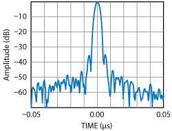
Figure 10 Matched filter compressor performance.
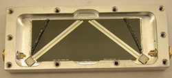
Figure 11 Phonon dispersive delay line.
Pulse compression results in the output signal-to-noise increasing by the bandwidth-time (BT) product. Assuming a lossless compressor, a signal of amplitude 1 and time length T will result in an output signal having amplitude (BT)½ and a time length of B-1. The resulting peak power gain is BT. Since noise does not correlate, its amplitude remains unchanged.
HARDWARE PERFORMANCE
Figure 11 shows the SAW dispersive delay line.1 The linear frequency modulated SAW compressor is fabricated on a yz-LINBO3 wafer and assembled in a 3" × 1.25" × 0.5" connectorized package. The compressor is centered at 331.8 MHz with a dispersive bandwidth (B) of 460 MHz and a time dispersion of 12.5 µs (T). For a 460 × 12.5 BT product without amplitude weighting, the resulting signal-to-noise gain is 37.6 dB. With a 50 dB Taylor weighted amplitude response, the output signal-to-noise ratio degrades 1.6 dB. The net signal-to-noise gain through the SAW compressor is then 36 dB; if the input chirp power level is at the noise level, for example, the compressed pulse peak is 36 dB above the noise.
Referring to Figure 11, the compressor is comprised of two slanted aperiodic interdigital transducers. The transducer buss bars are resistor terminated, balanced, microstrip transmission lines. With 140 percent bandwidth, harmonic suppression is important. Transducer interdigital electrode periods determine the frequency response harmonics. Unwanted input-output combined responses below the tenth harmonic are suppressed by using different transducer periods (electrode sampling) of 4 and 3 electrodes per wavelength. Good harmonic suppression requires tight line width control of the electrodes, whose periods vary from 0.72 to 5.7 µm.
Figure 12 shows the amplitude and phase vs. frequency responses of the SAW pulse compressor. In this iteration of the pulse compression system, the phase error has been well matched, but an amplitude error is responsible for the -35 dB symmetric sidelobes seen in Figure 10. A simple LC network can compensate for a smooth, low order amplitude error and reduce the time sidelobes to about -42 dB. SAW S-parameter data was obtained over an extended ambient temperature range from -40° to +80°C. Analysis of a discrete data set at ambient temperature increments of 20°C shows the SAW oven can be eliminated by compensating delay, slope and phase variation in the input chirp. Sensing the temperature of a non-ovenized SAW enables this compensation, reducing size, weight and power significantly.
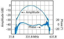
Figure 12 Measured response of the SAW pulse compressor (B= 460 MHz bandwidth, Taylor weighting), showing the phase response after removing the best-fit quadratic.
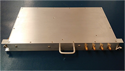
Figure 13 Highly matched pulse compression system.
Figure 13 shows the programmable waveform generator and the matched SAW compressor fully implemented in system-level hardware incorporating amplifiers and control electronics. The programmable digital waveform generator and the SAW pulse compressor enable a highly matched pulse compression system.
A second dispersive SAWs was also developed and described in the referenced article.1 The B/F center ratio of the 600 MHz SAW (B = 667 MHz) could be increased to 143 percent (B = 860 MHz). A 23.4 µs dispersion design fabricated on a 4 inch diameter wafer would result in a BT product of 20,000. It is practical to cascade two identical SAWs to achieve T = ~47 µs, a BT of 40,000 and a compression gain of 46 dB.
Reference
- Pierre Dufilie, Clement Valerio and Tom Martin, “Improved SAW Slanted Array Compressor Structure for Achieving > 20,000 Time-Bandwidth Product,” 2014 Ultrasonics Symposium Proceedings, pp. 201922022.