
Successful RF and microwave circuit design using active devices requires accurate modeling of nonlinear behavior. This is especially important in the telecommunications industry where nonlinear device behavior contributes to interference issues and a reduction in effective bandwidth.
Thus, a vendor agnostic, nonlinear behavioral model that accurately accounts for all of a device’s nonlinear effects and works with a variety of RF and microwave simulators is very valuable to designers. In fact, the focus on developing accurate nonlinear behavioral models has produced so many options that the nonlinear behavioral modeling world can be somewhat confusing. This article serves to bring some sense and structure to this space by presenting an overview of all the different nonlinear behavioral model types and comparing the effects they capture, the simulators they support, and the relative ease-of-extraction and distribution.
Modeling Domains
It is important to understand the two different RF and microwave simulation domains in which designers typically want nonlinear behavioral models to run. The first is standard circuit-level simulation, which includes linear simulation and nonlinear simulation technologies like harmonic balance, transient or SPICE, and circuit envelope techniques. With these simulation engines, the behavioral models can be formatted in either the time domain or frequency domain and the typical simulation output is voltage and current.
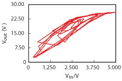
Figure 1 Nonlinear memory effects cause the current operation condition to be a function of the previous operating conditions.
The second option is that of system-level simulation, which usually involves a fixed time step time-domain simulator that commonly relies upon an underlying technology known as “data flow.” A more practical way of thinking about system-level simulation is to associate it with the creation and analysis of modulated signals or to think about the typical system-level simulation results such as error vector magnitude (EVM) — important for quantifying the performance of a digital radio transmitter or receiver — and adjacent channel power ratio (ACPR) — for determining the amount of spectral spreading.
Modeling Effects
Non-ideal effects typically seen in active circuits include both linear memory effects and nonlinear memory effects. Linear memory effects are simply the frequency-dependent behavior of an active device caused by linear capacitances and inductances. RF and microwave engineers have been dealing with linear memory effects for years, so they are not as exciting to designers these days as nonlinear memory effects.
Nonlinear memory effects, on the other hand, occur when the active device’s current operating condition is dependent on its previous operating condition. In other words, when a device starts to display hysteresis. One relatively straightforward way to see this is in an amplifier by looking at its AM to AM, or Vout versus Vin curves, where the input power level is swept up and down between random points. If there were no nonlinear memory effects present, the output would be the standard “smooth” AM to AM curve. However, in the presence of nonlinear memory effects, the result is a curve much like the one shown in Figure 1, where the trajectory taken to get from the starting input voltage to the final input voltage depends on the previous operating conditions of the amplifier. Nonlinear memory effects can be caused by a variety of sources, but the most common are low-frequency mixing products from the bias circuit, device self-heating and trapping.
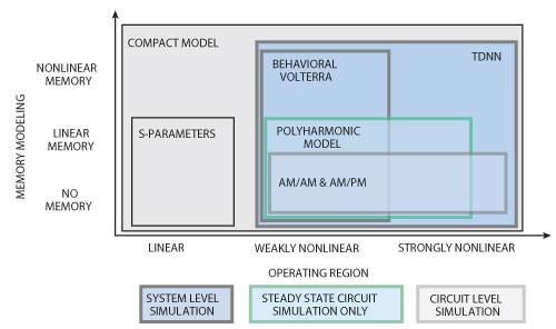
Figure 2 Types of models, including memory range and operating region range, and the relevant simulator technology.
Model Types
It is important to understand the different kinds of models that exist, the effects that they are capable of capturing and the simulators in which they work. The y-axis in Figure 2 shows model memory and ranges from those without memory effects — or a model that does not even capture frequency dependence — to those with fully nonlinear memory effects. The x-axis in Figure 2 describes the operating region of the device and spans from purely linear to strongly nonlinear, or in other words, very deep into compression for an amplifier. The different box colors indicate the simulator engines in which the models are most appropriate (converge to a timely and accurate solution).
S-parameter Models
S-parameter models are well known and widely used by almost all RF and microwave engineers. From the color and position of the S-parameter box in Figure 2, it can be seen that S-parameter models can be used with all circuit-level simulation engines, that they support linear memory or frequency-dependent behavior, and that they only model a linear device-operating region. This should be of no surprise to the RF and microwave engineer.
Compact Models
Compact models include Materka, VBIC, Angelov, BSIM3 and others. As shown in Figure 2, these models work with all of the circuit-level simulation engines and have the capability to capture all memory effects and cover all device operating regions. One important caveat is that an individual compact model will only be as good as the data from which it was extracted and the data ranges in which it was extracted over. Thus, the theoretical capability of a compact model might not be reflected in the ones that designers work with on a regular basis.
PHD Models
On the circuit-level simulation front, polyharmonic distortion (PHD) models include Agilent’s X-parameters®, S-functions, the Cardiff model and others. These nonlinear behavioral models are interesting in that from a user perspective, they seem to be S-parameters that also capture nonlinearities. In doing so, they cover an expanded device-operating region when compared to S-parameters. Presently, however, they are still limited to linear memory effects, or frequency-dependent behavior. In addition, they only really support steady-state or harmonic balance circuit-level simulation.
System Models
A standard way to represent an active device in a system simulator is with AM to AM and AM to PM curves. This approach is good in that it captures all the operating point nonlinearities, but it has limited linear memory effect capability and no nonlinear memory effect capability. The behavioral Volterra model, on the other hand, can capture all of the memory effects, including the nonlinear ones, but is somewhat constrained with regard to device operating region because of the practical limits on the number of model coefficients. Time delay neural network (TDNN) models, as Figure 2 shows, have the capability to handle all memory effects and all device operating regions, which makes these models very exciting from a system-level simulation perspective.
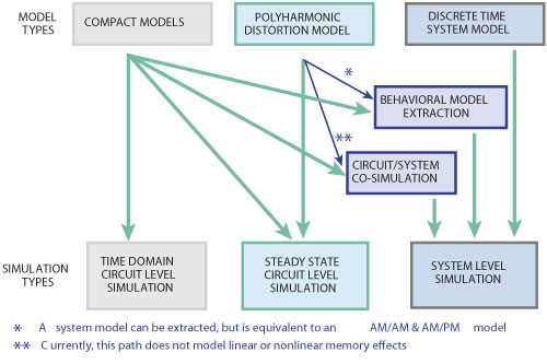
Figure 3 Simulator capability.
Simulator Compatibility
Although models are designed to work in a specific simulation engine or domain, there are often paths that will enable them to work in others as well. As shown in Figure 3, compact models work directly in time-domain circuit-level simulators and steady-state circuit-level simulators, but can also be used in system-level simulators through circuit-level co-simulation or behavioral modeling extraction. In fact, using some of the modeling definitions presented earlier in this paper, compact models can be extracted as AM to AM and AM to PM models, behavioral Volterra models or TDNN models for use in system-level simulation.
PHD models, on the other hand, are slightly more constrained. They only work directly in steady-state circuit-level simulators, and, while there are paths to use them with system-level simulators, there are a couple of issues to consider. The first is that when they are extracted as system-level behavioral models, the resulting behavioral model will always have the same model fidelity as the model from which it was extracted, regardless of its potential capability. Since PHD models do not model nonlinear memory effects, the resulting system models do not contain nonlinear memory effects. Another consideration is that when used in a co-simulation mode between circuit-level simulation and system-level simulation, neither linear nor nonlinear memory effects are considered due to the model formulation and the co-simulation engine characteristics.
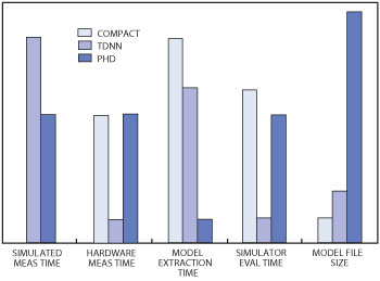
Figure 4 Comparison chart showing relative performance of compact, TDNN and PHD models.
Extraction and Distribution
So how do the models mentioned previously compare to one another with regard to extraction and distribution? The comparison chart in Figure 4 shows the relative performance of the compact model, TDNN and PHD models, including the time to gather enough simulation data to make the model, the time to measure enough data on the test bench to make the model, the time required to extract the model from the input data, the average target simulator evaluation time and model file size. With reference to both time and file size, it goes without saying that shorter and smaller are always better.
Observations
Simulated Measurement Time
For the compact model, the data input for the model extraction is always from a test bench and never from a simulation, so it does not have a simulated measurement time. The TDNN model needs modulated signal waveforms so it has a longer simulated measurement time than the PHD model, which uses a series of harmonic balance simulations as an input.
Hardware Measurement Time
With test bench hardware, however, things are a little different. The compact model and the PHD model require a fair number of measurements so they take relatively more time to measure than the TDNN model, which simply needs to capture modulated waveforms on a vector signal analyzer (VSA).
Model Extraction Time
Once the data is gathered for model extraction, compact models usually employ an iterative series of calculations and optimizations, which are relatively time consuming. The TDNN has a neural network that needs to be trained, which means there is some time investment involved, but overall it’s simpler than compact model development. The PHD model has a very low extraction time, in part because it is calculated as the data is being gathered so there are no explicit extraction steps that the model creator needs to run.
Simulator Performance
With regard to simulator performance, there is some apples-to-oranges comparison here, but in general compact models and PHD models run at the same speed, assuming that poorly formulated or poorly written compact models are not considered. The TDNN runs nearly instantaneously in system-level simulation (i.e., it runs at the same speed as any system level model).
Model File Size
For model file size, compact models are as good as it gets. They only require the storage of tens or hundreds of numbers. The TDNN model is also relatively compact, often generating files that are only tens of kilobytes. The PHD model, on the other hand, can quickly grow to become quite large. A model with 40 load and source impedance points, 10 input power points, 20 frequency points, three harmonics, and five source and drain bias points is approximately 2 GB. To make matters worse, for many devices, that number of points might not be sufficient.
Conclusion
The world of nonlinear behavioral modeling is fluid, complicated and, at least today, there is not a-one-size-fits-all solution to the problem. In a way, it could be compared to the Beta versus VHS debate of decades ago, but with a lot more options and a lot less capability overlap. Despite the confusion, however, there are still some important conclusions that can be drawn.
First, simulation tool support is very important. With all the model choices, designers need to be able to choose the model with the best availability and capability and know that their design tools will support it. Some companies support all of the models and the breadth of simulation engines as shown in Figure 2.
Second, PHD models, generally speaking, are in light demand at present as component-level simulation blocks, but not for discrete parts. Industry feedback is that this is due to file size issues, as previously mentioned, and the measurement and extraction complexity for adequate device models. Even for component-level simulation blocks, the lack of model fidelity when co-simulated with a system simulator presents an issue to designers trying to work with modulated signals or analyze system-level impairments. Compact models, although complex to create and not always formulated to maximize performance in a simulator, are very much the dominant model for circuit-level simulation.
Third, system-level modeling is a hot topic of late. As previously shown, there are several system-level models that offer more model fidelity in a system-level simulator than using circuit-level behavioral models in a system-level simulator. With the exception of S-parameters, system-level behavioral models are also much easier to extract from hardware than circuit-level models.
Lastly, it appears feasible to have a relatively simple test bench setup in a single PXI chassis that would allow any user to extract a TDNN model that handles all device operating regions and accounts for all nonlinear memory effects in a very reasonable amount of time and without any specialty model development knowledge. The advantage of a TDNN approach is not only a robust model but also an efficient model/solution within this domain.
While several solutions exist today that link RF and microwave design tools with test and measurement equipment, enabling engineers to produce a simulation model of their active device and providing the ability to build, test and validate design cases earlier in the product design cycle, more are surely on the way.