
Microwave thermal noise has long been employed for built-in test (BIT) of receivers and radiometers. Today’s compact solid-state noise sources are broadband and extremely stable making them very useful signal sources for a variety of tests. What is not commonly known is how many different types of BIT systems using noise currently exist. This article identifies these uses at the system architecture level and describes the differing attributes of the noise source required for each.
 | |||
| Fig. 1 Block diagram of a laboratory test set-up. | |||
 | |||
| Fig. 2 Spectrum analyzer display as the output of the test set-up. | |||
Perhaps the most common application using noise is to test the RF spectral gain/loss response of the front-end transmission line and microwave control componentry from the antenna through the RF receiver. System designers will sometimes use a switch to alternate between antenna and noise source; other times a directional coupler is used. The noise signal is required to have a bandwidth at least as wide as the receiver’s bandwidth. The receiver then detects the noise signal, which, in theory, is flat over the frequency band. If the detector is swept over frequency, the system will have the spectral data of its front end. The easiest way to see this in action in the laboratory is to simply use a spectrum analyzer (essentially a broadband swept receiver) and a front-end filter. Figure 1 shows a functional block diagram of a typical laboratory set-up. In this example, there are two switch settings, one where the noise is simply fed through the filter into the analyzer and the other in which there is an amplifier and bandstop filter inserted. The purpose of the bandstop filter is merely to simulate an amplifier gone partially bad. The outputs of the two switch settings are shown as two traces on the display of the spectrum analyzer shown in Figure 2. The spectral gain of the amplifier is then graphically visible as is the poor spectral gain response of the simulated flaw.
In a similar manner, an actual system during initialization, when the system is known to be functioning properly, would run the noise signal through the RF front end. The spectral values of a healthy system are then stored with an appropriate threshold window. Once deployed, if these values change during a BIT routine, a fault alarm will be triggered and switching to a back-up receiver may actually occur.
Injecting noise close to the antenna is a great way to determine if the overall system is healthy or not. However, if there is a problem, it is unable to discriminate which component is faulty. If this is important, then system architects will use a “drill down” design approach where the noise source is switched or coupled in at various places in the front end. By analyzing the output progressively closer to the down-converter, the system can more closely identify where the fault lies. The added complexity and cost of this approach is typically warranted for multi-antenna, redundant live back-up receiver hardware and/or when there are long networks of transmission lines from the antenna to the receiver hardware, such as found on a ship. The system architect needs to envision what is important for the system to be able to self-test and weigh this against the cost and complexity of integration of the BIT system.
One caveat is that noise sources in practice are never perfectly flat over frequency. This can be accounted for because they are inherently stable and the spectrum will not change significantly over time. It is important to start with the desired level of accuracy of the spectral response. If more or less a crude test is required, then little or no compensation is necessary. If a high degree of accuracy is required, then one of many compensation schemes can be employed.
One compensation method requires taking insertion loss data for a list of specific frequency points across the entire bandwidth of the receiver and storing them in a look-up table when the receiver is calibrated. Similarly, the spectral density (noise power normalized to a 1 Hz bandwidth expressed in dBm/Hz) is measured at the same frequencies and then stored in a table. With simple algebraic manipulation, software can “flatten” the response. In this manner, once the system is deployed, even subtle spectral changes in the receiver will be accurately detected. The complexity of this approach is more justified with wider bandwidth receivers since there is an inverse relation between flatness and frequency of not only the noise source but also the receiver. There begins to be a cost trade-off between trying to keep the front-end RF components, such as low noise amplifiers (LNA), attenuators and switches, as well as the noise source, super flat or having a more complex initial calibration. In today’s software dominated world, the cost of using software intelligently is making it cheaper and easier to utilize computer correction rather than paying huge amounts of dollars for very tightly specified RF componentry.
A common relative to the above application is a simple good/bad test used for systems, such as an X-band radar for missile guidance. It is mission critical that these systems are checked often, as it could be disastrous to launch a missile with a faulty guidance radar system. In these instances, a very fast system check is beneficial. In this manner, a noise source is switched on and the antenna off, and a noise “chirp” is sent into the receivers. The short chirp is controlled by sending a quick pulse into the bias supply of the noise source or using a TTL control if the noise source has an integrated TTL driver. An example of this type is depicted in the functional block diagram of Figure 3. In this diagram, the noise signal is coupled in to the RF front end. The noise eventually gets fed into a detector, which outputs a DC voltage based on the noise amplitude. This DC is sent to a comparator circuit that benchmarks it against a baseline value to decide if the system is healthy or not. The baseline voltage is established during system set-up in which the noise signal is initially sent through the system. Because the system during set-up is presumably in perfect working order, this measured DC value corresponds to a healthy system. This value is plugged into the comparator circuitry with an appropriate threshold.
 | ||
| Fig. 3 Block diagram of a radar system check set-up. | ||
In life or death situations, it is critical to check the health of the guidance system often. It is important that the monitoring is fast because during the test, the receiver may be effectively down. In the depicted example, the receiver can be checked in less than 1 µs. This is accomplished by means of synchronizing the TTL command to turn on the noise source to the detector.
Another common BIT performed using noise is a noise figure (noise temperature) test of the front-end receiver or LNA. Highly sensitive receivers employed to detect extremely weak signals require a very low noise figure front-end amplifier. If the LNA’s noise figure gets slightly worse over time, the entire performance of the receiver can become severely compromised. Noise figure is measured by injecting an accurately known amplitude of noise (Th) into a device under test (DUT) and finally into a receiver. This is compared with injecting ambient temperature noise (Tc) into the same set-up. This is done easily by turning the noise source on and then off. For the input noise temperature of Tc, the measured output noise power is referred to as N1. For the input noise temperature of Th, the measured output noise power is referred to as N2. These two noise powers, when expressed as a ratio, represent the Y-factor value given by

The noise figure is calculated from
NF(dB) = ENR(dB) – 10log10 (YFact–1) (1)
where
NF = noise figure
ENR = excess noise ratio of the noise source

A calibrated noise source will have a table of ENR values at spot frequencies across its bandwidth. The spot frequency points might be in 100 MHz or 1 GHz intervals, or sometimes the noise source is calibrated for ENR at the center frequency of a narrow band receiver. One thing that is clear from Equation 1 is that the accuracy of the noise figure measurement is only as good as the accuracy of the calibrated ENR value of the noise source. In addition, unlike laboratory noise figure measurements, there is typically some path loss between the noise source and the DUT, such as a switch network and a length of coaxial line. This path loss has to be accurately characterized and subtracted at each frequency point from the ENR table of the noise source. This process is commonly called “de-embedding.”
It should be noted that additional accuracy of the noise figure measurement is achieved by characterizing the complex impedance of the noise source, the input and outputs of the DUT, and the receiver, a technique called vector-error-correction. Systems such as radio-astronomy telescopes and the receivers of magnetic resonance imaging (MRI) machines that require extremely low noise figure front-end amplifiers commonly use this technique. The complexity of the mathematics underlying this is beyond the scope of this article, but there are many publications written on the subject for those who wish to pursue it further.
Once the parameters of the BIT are outlined, it is important to determine the attributes of the noise source for the design. The first and most obvious noise source parameter is simply the frequency band in which it is to be used. The next is the amplitude of the noise signal. For the cases of the spectral response and good/bad test, noise source attributes are similar. This article will describe these first. The most fundamental unit for noise amplitude is spectral density or noise power normalized to a 1 Hz bandwidth. In log form, the units are dBm/Hz. From this specification, the noise power can be calculated by adding the term 10log(BW), where BW is the bandwidth of a receiver. In general, the system will have a “sweet spot” amplitude where the detected noise signal is sufficiently above the noise floor of the detector but not so high that the signal is beyond the square law region of the detector or is saturating it. In addition, any control device or gain stage must be able to handle the output of the noise source. As an example, suppose that a system has a 20 dB coupler for injecting the noise, a 10 dB amplifier following the coupler and 6 dB of additional insertion loss going into the receiver. The receiver has a bandwidth of 100 MHz and ideally would like to receive a noise power of –40 dBm. To calculate the noise spectral density required by the noise source, the following equation is used
Noise Spectral Density =
–40 dBm –10log(100 MHz)
+20 dB –10 dB +6 dB
Noise Spectral Density =
–104 dBm/Hz (3)
The heart of today’s solid-state noise device is a noise diode. Special biasing circuitry is used to optimize the output for amplitude and flatness. A typical microwave noise diode from 10 MHz to 26.5 GHz generates a relatively small amplitude with values ranging from –150 to –140 dBm/Hz. To achieve an amplitude level such as required by the example above, about 40 dB of gain is required. In this case, a stand-alone amplified noise module can be used instead of trying to rig a separate noise source and amplifier(s).
Another attribute of a noise source is amplitude flatness over frequency. How flat a noise source should be for a system depends on a few factors. In narrow band devices, flatness is generally not a concern because noise sources are typically quite flat over a narrow band. In addition, the noise source manufacturer can optimize a noise source for a specific band to achieve a greater degree of flatness. In the wider band units, the importance of flatness depends on the overall system architecture. If an initialization procedure is used to establish a baseline level, flatness is a non-issue, so long as the noise spectrum does not change over time. Solid-state noise devices typically remain stable for a long period of time. As routine maintenance, the system should be re-initialized periodically to establish a new baseline. This is because there may be some slight drift in the noise source as well as other componentry over long periods of time (such as one year or more).
Some systems do not have an initialization procedure. In these, the noise baseline is factory established and hard-coded in. This puts much higher specification demands on the noise source (as well as other components) so that any source can be installed into any system. The trade-off here is complexity of logistics versus complexity of component specifications. As described earlier, software can be used to compensate for nonflatness.
It is also important to note that for systems that operate over a large temperature range, compensation circuitry can be employed to keep the noise amplitude at a set level. By the same token, voltage regulation circuitry can be utilized if there are likely to be drifts in the supply line. Noise sources are available with both built-in regulators and temperature compensation circuitry. Alternatively, noise sources can be characterized over a temperature range. This amplitude versus temperature data can then be loaded into a look-up table. The system then monitors temperature and pulls the appropriate ENR data, corresponding to the current temperature. By the same logic, ENR can be characterized over the power supply range and uploaded for compensation. Whether to use this approach or simply specify noise sources with regulators and temperature compensation circuitry is largely dependent on price and performance. If other parts of the system require temperature characterized data stored in a look-up table then it probably makes more sense to take this approach as the software algorithms and temperature sensor circuitry will already be in place.
The attributes of a noise source are determined by different factors in the case of the noise figure BIT. Frequency range and amplitude are the primary attributes. By convention, ENR is used to quantify its amplitude. ENR is easily converted to noise spectral density by the following equation
–174 dBm/Hz = 0 dB ENR (4)
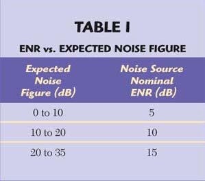
The optimum ENR of the noise source is dependant on the expected noise figure of the DUT. If the expected noise figure is high, the measured difference of the off and on noise source states will be too hard to discern accurately with the DUT’s comparatively large amount of self generated thermal noise. However, if the expected noise figure is very low and a high ENR noise source is used, then the measured values of the on and off states may have such disparate amplitudes that nonlinear dynamic range issues may compromise accuracy. Depending on how crucial the measurement uncertainty window needs to be, the designer can mathematically calculate the theoretical best ENR. This process can be mathematically exhaustive. Table 1 indicates a quick rule of thumb for ENR vs. expected noise figure. It should be noted that any path loss between the noise source and DUT must be accounted for. If a 10 dB noise source makes sense for the DUT but there is a 10 dB coupler and 3 dB of insertion loss, then a noise source with a 20 to 25 dB ENR is required.
 | ||
Maintaining a good match is extremely critical for noise figure measurements. High VSWR of the noise source will add to the noise figure measurement uncertainty. A typical 10 MHz to 26.5 GHz coaxial noise source used in the laboratory will have a very good match (1.35 max). This is fairly easy to achieve because the raw noise source generates an ENR of 25 dB allowing a 10 dB attenuator pad to follow it in the noise source assembly. The return loss of the noise source is twice the pad value, which corresponds to 1.22 VSWR, a low enough ratio for accurate measurement. However, when embedded in a system there may be 10 to 20 dB of loss in the noise path so an attenuator cannot be used. One way to achieve good VSWR in this case is by using a noise source with a built-in isolator. Of course the isolator also serves to protect the noise source from incident high power RF coming through the antenna.
Another important attribute is noise source calibration. The system must know the ENR of the noise going into the DUT. Some systems use a calibrated noise source in the system. Others will simply use an uncalibrated source and calibrate it during installation. An external ENR reference can be used during initialization. A commercially available laboratory calibrated noise source can work fine. In the case of radio-astronomy applications, some systems can use as a reference a known natural RF noise radiation standard such as the sun, or even a known temperature area of an ocean. These systems typically have an ultra sensitive radiometer, allowing the use of these precisely known but relatively low level RF noise energy sources as a reference. The disadvantage of using an external reference is complexity of architecture. The advantage is that using a reference calibrates the noise to the DUT so no further de-embedding is required.
Lastly, it is necessary to examine noise source flatness. Even a fairly nonflat noise source can be used provided there are enough calibration frequency points. The problem arises when it is necessary to interpolate between the calibration points. The uncertainty created by interpolation is larger as flatness degrades.
When designing a receiver BIT system, a multi-disciplined approach is required to achieve the best blend of cost, performance, design complexity and maintenance/calibration logistics. The architect must not only consider microwave design but also software, driver, metrology and mechanical design. The good news today is that there are many types of noise sources, complex noise module assemblies and noise calibration methods available to add to the architect’s design arsenal.
References
- G.W. Stimson, “Introduction to Airborne Radar,” Hughes Aircraft Co., El Segundo, CA, 1983.
- T.S. Saad, Editor, Microwave Engineers’ Handbook, Vol. 2, Artech House Inc., Dedham, MA 1971.
- T.M. Craig, “Noise Source Module for Microwave Test Systems,” US Patent 6,268,735 2001.
- S. Schneider, “Convert Specifications Between Competing Noise Sources,” Microwaves and RF, May 1987.
Patrick Robbins received his BS degree in interdisciplinary science from Rensselaer Polytechnic Institute in 1988. From 1989 to 1996, he was an applications engineer for Belt Technologies Inc., where, among other projects, he designed robotic power transmission systems for wafer fabrication equipment. In 2002, he joined KnowledgeXtensions, where he worked in developing new applications for its Java/XML-based e-learning software platform. He is currently director of the Noise Products Group at Micronetics Inc., Hudson, NH.