
At RF and microwave frequencies, a real-life surface-mount multilayer ceramic capacitor (MLCC) behaves differently from an ideal capacitor. This difference can be attributed to the internal parasitic elements associated with real-life components. As a result of these elements, MLCCs typically exhibit resonances at specific frequencies. External aspects, such as the substrate and the dimensions of the solder pads on the printed circuit board (PCB), also influence performance. To accurately simulate the behavior of a real-life capacitor, a suitable model is required. One solution for capacitor models comes from Modelithics, which offers equivalent-circuit models for capacitors, inductors and resistors from many manufacturers. These models, known as Microwave Global Models™, scale with respect to part values, substrates and solder-pad dimensions. By using these models, it is possible to observe how these resonances depend on factors such as case sizes, substrates and solder-pad dimensions.
CAPACITOR BASICS

Figure 1 (a) Ideal 1.5 pF model, (b) simplified model of a real-world 1.5 pF and (c) the Modelithics Microwave Global Model for the YAGEO CQ0100 capacitor series.
Ideal capacitors differ from real-life capacitors in multiple ways. Figure 1 shows a simple project in Keysight Advanced Design System (ADS) that includes both an ideal 1.5 pF capacitor model (Figure 1a) and a simplified model of a real-world 1.5 pF capacitor (Figure 1b). This simplified model is a frequently used representation that includes the nominal capacitance, equivalent series resistance (ESR) and equivalent series inductance (ESL). It is referred to as a simplified model because a real-world MLCC has additional elements that are not included in this model. The project shown in Figure 1 also consists of the Modelithics Microwave Global Model for the YAGEO CQ0100 capacitor series (Figure 1c).
Since an ideal capacitor is simply a pure capacitor with no additional elements, its total impedance is equal to the capacitive reactance given by Equation 1:

where:
f = frequency (Hz)
C = capacitance (farads)
The total impedance of the simplified real-world capacitor is given by Equation 2:

where:
ESR = equivalent series resistance
XL = inductive reactance (from the ESL)
XC = capacitive reactance (from the nominal capacitance)
Note that inductive reactance is given by Equation 3:

where:
f = frequency (Hz)
L = inductance (henries)
SIMULATING THE SELF-RESONANT FREQUENCY
In Figure 1, the simplified real-world capacitor has a nominal capacitance of 1.5 pF along with an ESR of 580 mΩ and an ESL of 0.19 nH. The simplified real-world capacitor is a series RLC circuit. For a series RLC circuit, the capacitive reactance and inductive reactance have an equal magnitude at a specific frequency. This frequency, known as the resonant frequency, is given by Equation 4:

Hence, a capacitor has a resonant frequency of the same form. This frequency, known as the capacitor’s self-resonant frequency (SRF), is given by Equation 5:

The SRF decreases as the capacitance increases. Additionally, the capacitive reactance and inductive reactance have equal magnitude at the SRF. Hence, at the SRF, the total capacitor impedance reaches a minimum value that is simply equal to the ESR (as shown in Equation 2). Equation 5 is used to calculate an SRF of approximately 9.4275 GHz for the simplified real-world 1.5 pF capacitor shown in Figure 1.
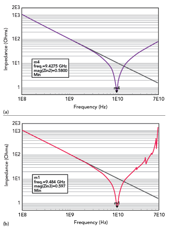
Figure 2 (a) Impedance of the ideal capacitor (black trace) and the simplified capacitor model (purple trace). (b) Impedance of the ideal capacitor (black trace) and the Modelithics model (red trace).
Modelithics models capture substrate-dependent parasitic behavior and offer advanced pad features, among other capabilities. The CQ0100 series is an MLCC series (01005 size) that covers a capacitance range of 0.1 to 15 pF. The Modelithics CAP-YAG-01005-001 model is validated by measurements performed up to 67 GHz. The model covers the full range of part values for the CQ0100 series.
In this model, the capacitance value is 1.5 pF, and it uses a 4 mil thick Rogers RO4350B substrate. The dimensions of the solder pads are the default values for the length, width and gap (7.3, 8 and 5.1 mils, respectively).
Figure 2 shows the simulation results comparing the impedance of the ideal 1.5 pF capacitor to the simplified real-world 1.5 pF capacitor model (Figure 2a) and the impedance of the ideal 1.5 pF capacitor to the Modelithics model for the 1.5 pF CQ0100 capacitor (Figure 2b). For the simplified real-world capacitor, the impedance is equal to the ESR (580 mΩ) at the SRF (9.4275 GHz), and the 1.5 pF CQ0100 capacitor exhibits an SRF of 9.484 GHz.
The results show that the simplified real-world 1.5 pF capacitor and the 1.5 pF CQ0100 capacitor do not behave like ideal capacitors. In the case of the ideal capacitor, the impedance only decreases as the frequency increases. The real capacitor follows the impedance curve of the ideal capacitor up to a certain frequency, then deviates. Specifically, the impedance decreases more sharply as it approaches the SRF. At the SRF, the impedance reaches a minimum value. Above the SRF, the impedance increases as the frequency increases.
Continuing further, a real capacitor’s total impedance is capacitive below the SRF, as the capacitive reactance is greater than the inductive reactance. Above the SRF, the total impedance is inductive, as the inductive reactance is greater than the capacitive reactance. In other words, above the SRF, the capacitor behaves like an inductor. Thus, a capacitor acts as a “DC blocking inductor” above the SRF.1
As shown in Figure 2, a real capacitor does not exhibit the same behavior as an ideal capacitor. However, comparing the behavior of the simplified real-world 1.5 pF capacitor with the behavior of the 1.5 pF CQ0100 capacitor reveals more information. In Figure 2, the impedance of the 1.5 pF CQ0100 capacitor resembles the impedance of the simplified real-world capacitor model. However, above the SRF, there are some noticeable differences. Specifically, the 1.5 pF CQ0100 capacitor exhibits impedance spikes at several frequencies above the SRF. Figure 3 demonstrates an S-parameter simulation of this same Modelithics model for the 1.5 pF CQ0100 capacitor in a two-port series configuration. Figure 4 shows the simulated S21 results. For comparison, Figure 4 also shows S21 after performing the same S-parameter simulation of the ideal 1.5 pF capacitor.
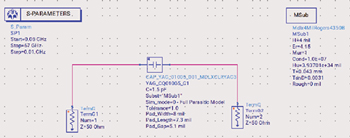
Figure 3 ADS schematic used for an S-parameter simulation of the capacitor.
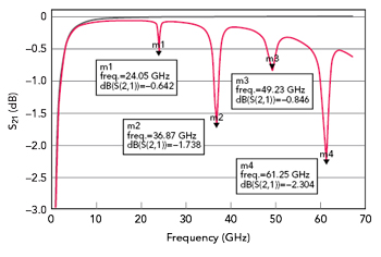
Figure 4 Red trace: Simulated S21 of the CQ0100 capacitor. Black trace: S21 of an ideal capacitor.
In Figure 4, the simulated S21 of the 1.5 pF CQ0100 capacitor exhibits distinct attenuation notches at the same frequencies where the impedance spiked. These attenuation notches represent the parallel resonant frequencies (PRFs) that appear due to the parallel parasitic elements of an MLCC. These PRFs can also be referred to as higher-order resonances, as an MLCC has a first PRF, a second PRF, a third PRF, etc. In this case, the first, second, third and fourth PRFs are at 24.05, 36.87, 49.23 and 61.25 GHz, respectively. Therefore, while the simplified model of a real-world capacitor may be effective to some degree, it is not a complete representation of a real-world MLCC because it omits the parallel parasitic elements.