

Modern radar systems, as demonstrated in Figure 1, are increasingly embedded within complex, multi-domain platforms—from airborne surveillance and automotive sensing to joint radar-communications systems. Therefore, designers must navigate a wide variety of technical trade-offs to ensure performance, efficiency, and integration.
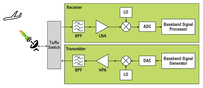
Figure 1 Typical radar architecture.
While radar theory is well established, the challenge today is bridging the gap between high-level performance requirements and component-level design choices. The radar range equation serves as a foundational tool for making this connection. Still, its effective use demands an understanding of system-level objectives and practical limitations of real-world sub-systems and components. Originally developed during World War II to support radar performance assessment, the equation remained classified until after the war, when it became publicly available and widely adopted.
Since then, the radar equation has evolved to incorporate correction factors to enhance its accuracy and applicability for complex environments and modern radar systems. Comprehensive treatments, such as those found in (Barton, 2013), provide detailed formulations to improve range predictions and support the design of contemporary systems.
As a design tool, the radar equation enables system dimensioning and facilitates trade-off studies involving transceiver characteristics, range, and resolution. It supports informed design choices and prevents over-design and under-design, which can lead to excessive development cycles and cost increases.
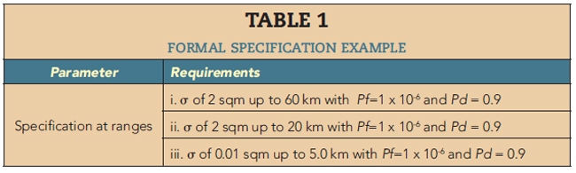
An example of a technical section of a radar procurement document or request for proposal is shown in Table 1. One of the most important parameters is range, typically written as “shall be able to detect a target of minimum radar cross section, σ=σ0, at distance R=R0 km with Pƒ=Pƒ0 and Pd=Pd0”, where Pƒ and Pd are the probability of false alarm and detection, respectively. Other performance requirements can include the number of targets, range resolution and acquisition timing.
Radar Range Equation
For this evaluation, only strictly required mathematical derivations are provided, as the emphasis is on usability. Analysis is restricted to thermal noise being the dominant source of interference.
While the emphasis is on pulsed radar systems, radar waveforms and architectures vary widely, including continuous wave (CW), frequency-modulated CW (FMCW) and pulse-Doppler systems. However, this diversity does not diminish the value of a top-down systems design approach, which remains applicable across radar modalities.
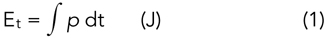
To begin, consider pulse energy, peak power and pulse duration. The pulse energy Et is equal to the integral of the instantaneous power p over the interval of time occupied by the pulse, i.e. the pulse duration:
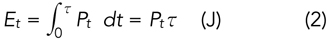
For a constant transmit pulse Pt of duration τ seconds, the instantaneous power would equal the peak power Pt so the pulse energy would be:
By applying Et to the input of a matched isotropic radiator, the energy per square metre at distance R from the transmitter is given by:
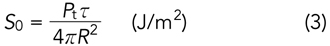
Gt represents the gain of the transmit radar antenna relative to the isotropic reference, so:
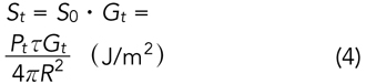
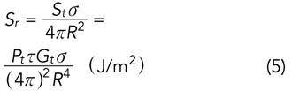
The radar cross section (RCS), denoted by σ, quantifies the “effective echoing area” of a reflective object or target. If the target is in the direction of maximum radar antenna gain Gt at distance R, the total energy per square metre reflected by the target covering a sphere of radius R centred at the target is:
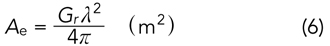
The receiver antenna effective aperture Ae represents the ability of a receiving antenna to collect incident electromagnetic energy from a given direction:
Thus, the total received energy referenced at the output terminal of the receiver antenna can be expressed as:
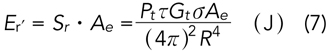
Combining Equations 6 and 7, the received energy at the output terminal of the receiver antenna can be given by:
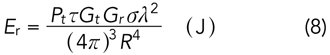
This expression makes explicit the dependency on the carrier frequency  and the receiver antenna gain Gr. It shows that the physical size of the antenna and the transmitted waveform characteristics (pulse duration τ) contribute to the received energy.
Rearranging Equation 8 yields the range equation, expressed in terms of received energy:
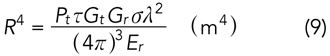
This form is particularly useful when evaluating radar systems based on required detection energy thresholds. If the received energy Er is reduced to the minimum detectable level Er,min, and the corresponding range is defined as the maximum detection range Rmax, then Equation 9 becomes:
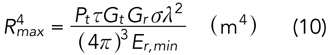
This is the maximum radar range equation: the theoretical upper limit of detection range under ideal conditions.
The available thermal noise power generated at the input of an ideal receiver at systems equivalent temperature Ts and noise bandwidth B is:

Where k is Boltzmann’s constant (1.38×10⁻²³ m2.kg.s-2.K-1). The bandwidth B of a superheterodyne receiver is taken to be the bandwidth of the IF amplifier or matched filter. Although the noise bandwidth is not strictly equal to the 3 dB bandwidth, in many practical applications the 3 dB bandwidth is a sufficient approximation which simplifies calculations without significantly impacting range estimations, especially for well-matched filter designs.