
While asynchrony is difficult to depict, Figure 5 shows a qualitatively similar graph where the aforementioned processing units are assigned to each devices’ ‘capture stream’; by looking at the number of executed test iterations, one sees that the throughput has significantly improved when compared against both previous cases. However, this does not necessarily mean that the processing of the capture data coming from a specific device is also handled by a specific processing unit.
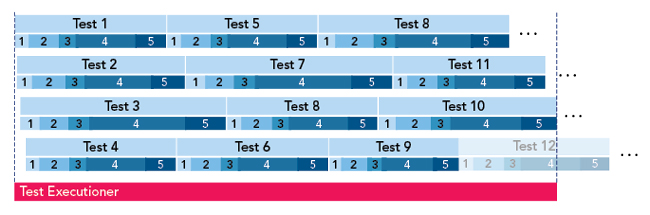
Figure 5 Strongly parallelized operation with ‘sorted’ operators.
It should be mentioned that parallel data delivery is not always possible: in cases where single DUTs are tested, it may not be possible to add multiple capture devices (such as spectrum analyzers) due to complex RF connectivity or instrumentation.
TEST RESULTS
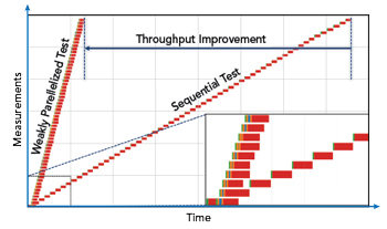
Figure 6 Comparison of sequential (right) and weakly parallelized (left) test execution. Lower right shows the first few steps.
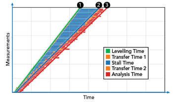
Figure 7 Throughput subtask segmentation and the respective effect on the overall systems’ performance.
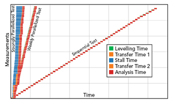
Figure 8 Performance of strongly and weakly parallelized tests vs sequential test.
To verify the benefits of parallel test execution, a realistic scenario often found in 5G applications was set up and executed in multiple test configurations. The setup allowed two modes, a sequential and a weakly parallelized operation. The specific test system consisted of the signal generator (R&S SMBV100B), spectrum analyzer (R&S FSVA3000) and R&S server-based testing (SBT) unit, a processing platform capable of processing 16 data sets in parallel. The SBT was configured so that EVM, ACLR and SEM metrics were calculated in each test iteration. The generator was set up in such a way that the stimulus output power was stepped across 59 different levels. The analyzer was set up so that data was captured and transported as I/Q data files. The connectivity between devices was given through a local gigabit Ethernet with no special hardware used to interface the participating devices. All calculations were compared to ensure validity of the results.
Figure 6 depicts the qualitative results of the two scenarios. It confirms that the performance in a sequential operation (shown in Figure 6 on the right) is limited by individual test step execution time. The lower right diagram is a zoom-in into the first few test steps executed, depicting the difference between sequential (flat) and parallel (steep) approaches. A breakdown into individual subtasks within each step is irrelevant since all test steps have a largely consistent duration. Total test time for all 59 steps is simply the sum of individual test execution periods.
The left part of the diagram depicts the weakly parallelized operation with a single analyzer being operated as the sole capture data source. The zoomed-in view on the lower right shows the first 10 iterations of the parallel and 8 iterations of the sequential test. It illustrates how each individual test step, divided in subtasks, is being executed. The parallel execution of analysis task is reflected by the overlapping red bars. One can also notice that the single-device operation results in the test preparation and data capture subtasks effectively determining the systems performance. This is a result of having both fast data transfer capabilities and enough parallel processing units available.
By quickly inspecting the difference between the two scenarios in total test execution time in Figure 6 (dashed vertical lines), one clearly sees that the performance gain in the second scenario is substantial; the weakly parallelized setup performs almost six times faster than the sequential test. This can be considered a significant improvement for any scenarios requiring acceleration of repetitive test execution. In contrast, the ratio of used equipment is almost at 100% for the duration of the test. The ratio in sequential execution is lower than 10% on average for the complete test sequence.
A general view at the system’s performance can be seen in Figure 7. Here, a system was purposely configured with a low number of parallel processing units and used to run the same test. The system’s throughput performance data was recorded, with the separation of individual phases in each test step. First phase (green) is the analyzer preparation time where input levelling is performed; second phase (orange) is the data capture and transfer time to a centralized buffer. Third phase (blue) is a file server that is utilized as a buffer. Fourth phase is the data transfer to the processing unit, whereas phase 5 (red) is the actual processing of the capture.
By observing the diagram, one can identify three segments that have an effect the performance:
Segment 1, identified by the green gradient No 1 in Figure 7, defines how fast data is delivered. Speed improvement is done by both acceleration of data delivery and parallelization of data sources where applicable. This is a large factor to the speed of the system but is often limited by the test setup or physical boundaries.
Segment 2, which is the area between gradients 1 and 2, reflects how much a system must wait (or buffer) due to a lack of parallel processing capabilities. In cases where enough processing units are available at the system’s disposal, the blue area is minimized. This segment can be considered as both the biggest contributor to overall performance and the easiest to tune, if the underlying platform supports such scalability. In this test case, SBT is specifically designed to support an arbitrary number of processing units running on single hardware unit (e.g. server) or across multiple units.
Segment 3, the red area between gradients 2 and 3, defines how fast individual processing units can execute the analysis task. Optimizing a single processing time has a comparatively small effect on the overall system’s performance and can be generally deemed as an expensive tuning factor.
In additional tests, strong parallelization was approximated by a simulation of an arbitrary number of capture devices, effectively resulting in an almost-immediate availability of capture data. The latter use case functions as a setup allowing an estimation of best possible performance of the processing platform. It shall be considered a borderline, yet real scenario, where enough data capturing devices is available. Figure 8 shows the strongly parallelized test simulation in comparison with the other two scenarios.
CONCLUSION AND OUTLOOK
As expected, the strongly parallelized test performs the best. Due to the system’s configuration of 16 parallel processing units, the blue segment shows where buffering takes place since data is almost instantaneously available for processing. Adding further processing units would have minimized the overall throughput time to a minimum, effectively rendering improvement factors of 10 and more versus sequential testing.
Note that data-transfer phases in both Figures 7 and 8 (in orange) have a little impact on the system’s performance despite some variance in the duration. This is a typical observation when a non-deterministic transfer protocol (such as TCP over Ethernet) is used. Yet, the asynchronous, non-blocking operation can support such an execution mode.
The asynchrony is enabled through the utilization of system components that are commonly used in scalable IT systems. The recent rise of cloud-based systems, both public and on-premises, render the usage of such building blocks possible for system designs beyond the original use case. Here, the SBT solution tested is built around such scalable components. Yet, it is a purely localized deployment with no external connectivity requirements.
The benefits of such a solution with a focus on throughput improvements are manifold: apart from the discussed faster overall test speed or throughput, parallelization renders better equipment utilization ratios possible and allows a high ROI. Eventually, new usage-based commercial models become more attractive in cases where lower upfront investment in high-value equipment is desired.