
One might ask why engineers should expand their S-parameter measurement practices to include uncertainties, since they have been largely ignored until now. The answer lies mainly in the advancement of technology: as new technologies emerge and are introduced as standards, the specifications and requirements for products get tighter, especially with increasing frequency. This trend can be seen not only with systems, but also at the component level, including amplifiers, filters and directional couplers. Therefore, engineers responsible for the design and production of these components need to increase the confidence in their measurements and product characterization.
Imagine the following: an engineer designs an amplifier requiring a minimum gain over a frequency bandwidth. The amplifier is measured and meets the specification. A few hours later, the amplifier is remeasured and no longer meets the specifications at the high end of the frequency band (see Figure 1). Why is the amplifier not meeting the specification? There could be many reasons: the measurement system drifted, someone in the lab moved or damaged one of the cables in the measurement setup or one of many other possibilities, including doubts about the design, fabrication or stability of the product.
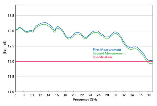
Figure 1 Amplifier gain measurements at two times: the first in spec, the second out of spec at the upper band edge.
If it is that easy to take two measurements and obtain different results, how can one know which measurement is correct? The confusion arises from not characterizing and including the uncertainties in the measurement, which ultimately leads to an overall lack of confidence in the results. Careful engineers use methods to validate a setup before taking measurements. More careful users test “golden devices” - those with similar characteristics to the actual device under test (DUT) - as a validation step and reference internal guidelines to decide whether the data is good enough. While this is a step in the right direction, how are these guidelines defined? Are the guidelines truly objective, or is subjectivity built in? How close is close enough? Uncertainty evaluation is a powerful tool allowing users to both validate vector network analyzer (VNA) calibration and properly define metrics for golden devices before taking measurements. Figure 2 illustrates this, showing the same amplifier gain measurement with the uncertainties of the system.

Figure 2 Amplifier gain measurement showing measurement uncertainty, calculated using Maury MW Insight software.
Uncertainties
Every measurement, no matter how carefully performed, inherently involves errors. These arise from imperfections in the instruments, in the measurement process, or both. The “true value of a measured quantity” (atrue) can never be known and exists only as a theoretical concept. The value that is measured is referred to as “indication” or (aind), and the difference between the true value and the measurement indication is the error:
Since the true value is unknown, the exact error e in the measurement is also unknown. There are two types of errors:
Systematic errors: In replicate measurements, this component remains constant or varies in a systematic manner and can be modeled, measured, estimated and, if possible, corrected to some degree.1 Remaining systematic errors are unknown and need to be accounted for by the uncertainties.
Random errors: This component varies in an unpredictable manner in replicate measurements.2 Some examples are fluctuations in the measurement setup from temperature change, noise or random effects of the operator. While it might be possible to reduce random errors - with better control of the measurement conditions, for example - they cannot be corrected for. However, their size can be estimated by statistical analysis of repetitive measurements. Uncertainties can be assigned from the results of the statistical analysis.
In general, a measurement is affected by a combination of random and systematic errors; for a proper uncertainty evaluation, the different contributions need to be characterized. A measurement model is needed to put the individual influencing factors in relation with the measurement result.3 Coming up with a measurement model that approximates reality sufficiently well is usually the hardest part in uncertainty evaluation. Propagating the uncertainties through the measurement model to obtain a result is merely a technical task, although sometimes quite elaborate. Finally, the measurement result is generally expressed as a single quantity or estimate of a measurand (i.e., a numerical value with a unit) and an associated measurement uncertainty u. This procedure, described here, is promoted by the “Guide to the expression of uncertainty in measurement” (GUM),4 which is the authoritative guideline to evaluate measurement uncertainties.
S-Parameters and VNA Calibration
How do these concepts apply to S-parameter measurements? Recall that S-parameters are ratios of the incident (pseudo) waves, denoted by a, and reflected (pseudo) waves, denoted by b:

The definition of S-parameters implies a definition of reference impedance.5-6 The most common measurement tool used to measure S-parameters is a VNA. While different VNA architectures exist, the most common versions for two-port measurements use either three or four receivers.5-7
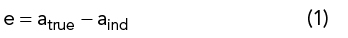
To simplify the understanding of the subject, consider a one-port VNA measurement (see Figure 3). The case for two-port or more general N-port measurements can be obtained through generalizations, as shown in the literature.7 Figure 3a shows a typical setup, where a VNA, cable and connectors are used as a measurement system to measure a DUT. To evaluate uncertainties in the S-parameter measurements, a measurement model first needs to be established, to describe the relation between the output variables, the incident and reflected waves at a well-defined port (i.e., the reference plane), and the indications at the VNA display (i.e., the raw voltage readings of the VNA receivers). These models should include systematic as well as random errors to increase confidence in the results. Not estimating systematic errors correctly leads to inaccurate measurements. On the other hand, wrong estimates of the random errors can either degrade the precision of the result or indicate the results are precise when they are not.
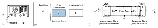
Figure 3 One-port measurement hardware setup (a), systemic error model (b) and signal flow graph (c).
Classical VNA Error Model
VNA measurements are affected by large systematic errors which are unavoidable and inherent to the measurement technique, related to signal loss and leakage. They establish a relation between the indication (measured)

and the S-parameter at the reference plane

shown by the signal flow graph of Figure 3c. The error box consists of three error coefficients: directivity (E00), source match (E11) and reflection tracking (E01). The graphical representation in Figure 3b can be transformed into a bilinear function between the indications and S-parameters at the reference plane through the three unknown error coefficients. To estimate the unknown error coefficients of the model, three known calibration standards must be measured for the one-port case, more if multiple ports are involved. After estimating the error coefficients, any subsequent measurement of raw data (i.e., indications) can be corrected. This technique is commonly referred to as VNA calibration and VNA error correction.
Different calibration techniques have been developed to estimate the error coefficients. Some require full characterization of the calibration standards, such as short-open-load (SOL) or short-open-load-thru (SOLT), while others require only partial characterization, such as thru-line-reflect (TRL), short-open-load-reciprocal thru (SOLR) and line-reflect-match (LRM) for two-port calibrations.8 Even if the calibration standards are characterized, they are not perfectly characterized, and the error associated with the characterization will increase the inaccuracy of the estimated error coefficients: directivity, source match and reflection tracking.
Engineers have developed experimental techniques to estimate these residual errors (i.e., residual directivity, residual source match and residual reflection tracking). Connecting a beadless airline terminated with a reflection standard to the calibrated port enables the residual errors to be observed as a superposition of reflections versus frequency. In the frequency domain, this implies ripples in the reflection coefficient (see Figure 4). Due to the characteristic pattern in the frequency response, the method is referred to as the “ripple method,” where the magnitude of the ripples is used to estimate the residual errors and uncertainties related to directivity and source match. This method has various shortcomings: it is unable to determine the residual error in tracking and requires handling air-dielectric lines, which becomes impractical as frequency increases.7
Figure 4 Source match after one-port calibration using Maury MW Insight software.
Residual errors have been used to gain confidence in the measurement based on experience. The challenge is to understand what a residual directivity of 45 dB means if a DUT with 36 dB return loss is measured. However, the uncertainties of the error coefficients are not reliable when estimated with the ripple method, and they are insufficient to gain confidence in the measurement results. The classical VNA error model is thus incomplete to perform VNA calibration and VNA error correction with uncertainty evaluation.
Adding Uncertainties to the Classical VNA Error Model
This section explains how to expand the classical VNA error model into a full measurement model by adding the other factors influencing the measurement. Using such a full model, the uncertainties can be evaluated in a direct and conceptually clear method. The measurement setup leading from the calibration reference plane to the receiver indications contains several sources of error and influence factors that contribute to the total uncertainty. The classical VNA error model can be expanded to include these factors, becoming a full measurement model. Typical components include the VNA (e.g., linearity, noise and drift), cables, connectors and the calibration standards. The European Association of National Metrology (EURAMET) recommends the model shown in Figure 5, where the traditional error coefficients are identified by the E block and the other influence factors represented by the R, D and C blocks.7,9 The full model in the figure contains just the building blocks, which are further refined using signal flow graphs. Without going into the details of these models, the main errors and related signal flow graphs are described.
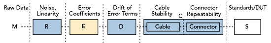
Figure 5 VNA measurement model.
Cable and Connector
Cables are used between the reference plane and the receiver indications, making them part of the calibration. They are subject to environmental variations, as well as movement and bending. When cables are moved or bent during calibration or DUT measurement, the error coefficients are expected to change. The cable model uses two parameters: cable transmission (CAT) and cable reflection (CAR), shown in Figure 6a. While cable suppliers typically specify these values in cable assembly datasheets, the cables should be characterized for the typical range of flexure or movement during calibration and measurement.7
Similarly, the connectors used for connecting and disconnecting the calibration standards and DUT affect the reference plane, based on how repeatable the pins and fingers are designed and built. The S-parameter response of a device differs each time it is connected, disconnected and reconnected, which is modeled by one parameter, the connector repeatability (COR).
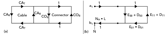
Figure 6 Models for the cable and connector (a) and VNA noise, linearity and drift (b).