

A parameterized meandered-line dipole antenna on FR4 substrate with complex chip impedance was studied. Five geometric parameters are considered:
- Meander amplitude, H
- Conductor width, W
- Meander spacing, S
- Feed gap, G
- Length of the first meander leg, H0.
The key objective was to minimize |S11| < -20 dB at 915 MHz or alternatively, minimize S11 over a specified frequency range.
Other things can be optimized if needed, for example:
- Maximize realized gain > 6 dBi
- Achieve a hemispherical far-field distribution pattern
- Favor designs with larger feature sizes (> 0.5 mm) for manufacturing ease.
RFID tags contain a small chip that is used to activate the tag. Chip impedance is an important variable in tag design. In this example, the chip resistance Rc is 11.5 Ω and the capacitance Cc is 3 pF. Lower chip resistance tends to make matching more difficult. The goal is to design an antenna whose natural impedance is a conjugate match for the chip impedance. The complex chip impedance is shown in Equation 1.
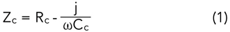
So, the antenna needs to have an inherent impedance (Equation 2).
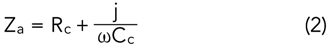
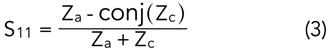
The S-parameter, the quantity to minimize close to the target frequency of 915 MHz, is given by Equation 3:
The basic layout of the tag is shown in Figure 1. The geometric features are adjusted and optimized until the antenna meets the performance requirements. The S-parameter plot for these nominal initial values is shown in Figure 2. The initial design does not meet the performance specification or have the correct resonant frequency.
Figure 1 Example geometry of a miniaturized single-port meandered-line dipole antenna.

Figure 2 S-parameter vs. frequency for an arbitrary initial starting point.
Using LHS, 300 COMSOL frequency sweep simulations are performed (average 3 minutes each on a 32-core workstation, total ~15 hours). The 15-hour simulation time is chosen intentionally, as one can set the model solving at the end of the workday and have the results available for processing the following morning.
RESULTS AND INTERACTIVE EXPLORATION
Once the surrogate model has run, the data can be used to train a deep neural network. When trained, the result is a function that can be evaluated using frequency and the geometric inputs. The function form is thus shown in Equation 4.

Here, the first five inputs are the geometric parameters, and fr is the range of frequencies over which to evaluate. Evaluation of this function for different combinations of parameters is practically instant, as a weighted sum (from the weights and biases computed during training) is evaluated under the hood.
The evaluation, result display and convenient method of changing input parameters (using a slider which updates the results and geometry plot in real-time) can be packaged into a simple and intuitive user interface using the COMSOL Application Builder. The app also has a “Verify Results” button in the ribbon. This allows the full FEA solution to be computed once an interesting result has been obtained. This is a crucial step when using this technique; the full model should always be computed for verification purposes.
The interactive dashboard provided by the app allows cross-functional teams to filter designs by constraints (e.g., cost proxies via material volume) and select candidates for prototyping.
OPTIMIZATION
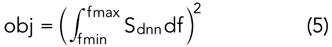
Manual tuning of the parameters, while instructive, can be time-consuming, even when just running inference from the surrogate model. Optimization running on inference can compute global minima for a suitable objective function. In this case, the S-parameter is minimized over a user-selected frequency range. The objective function is shown in Equation 5.
The parameter space of antenna configurations can contain many local minima, but only one true global minimum. COMSOL includes an efficient global optimization (EGO) solver, which can compute a true global minimum. Running this for different objective functions can quickly generate a desirable starting point, which can be manually tweaked given the practical design issues discussed earlier.
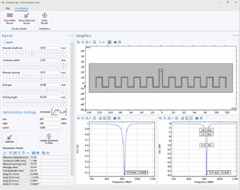
Figure 3 Screenshot of the app, which allows rapid tag design iteration.
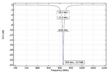
Figure 4 Optimized S11 plot for the antenna design, showing resonance frequency and bandwidths at -3, -5 and -10 dB.
The screenshot in Figure 3 shows a result that was first computed using the optimization, then tweaked slightly to get the minimum at exactly 915 MHz. The frequency range in which to optimize is specified in the user interface. If a high bandwidth is required, the frequency limits can be expanded. If the main goal is to have the smallest S-parameter at exactly 915 MHz, the window can be shrunk to a very small value. The user can quickly see the tradeoffs in geometrical footprint and performance given their target specification.
An added benefit to this approach is that derivatives of the objective function can be computed purely from the inference. This allows the sensitivity of the S-parameter with respect to each geometric parameter to be quantified. These values indicate which of the dimensions will affect performance the most if the exact values are not met during manufacturing. These can be explored further using uncertainty quantification, if needed.
The optimized result for a frequency range of 910 to 920 MHz is shown in Figure 4. The antenna meets the target of -20 dB and the resonance is at exactly 915 MHz. Expanding the frequency integration range would result in slightly different solutions, with the antenna obtaining a higher bandwidth, but the frequency at which the S-parameter is minimized might be slightly away from 915 MHz.
Note: Running optimization on the full FEA model would require an inordinate number of solutions to be computed, limiting runs to overnight or possibly over weekends. Crucially, if the objective function changes, the optimization needs to be re-run.
DISCUSSION
This workflow shifts antenna design from simulation-constrained iteration to data-driven collaboration. Surrogates democratize access, enabling product managers to quantify tradeoffs early. The simple RFID case demonstrates practical benefits: identifying manufacturable designs without sacrificing core performance.
Limitations include initial data generation cost (mitigated by cloud and batch compute) and surrogate validity only within training bounds.
CONCLUSION
Neural network surrogate models trained on COMSOL Multiphysics simulation data enhance and speed up antenna design and development. By enabling millisecond evaluations, this approach facilitates interactive exploration, rapid robustness analysis and balanced decision-making across electrical and practical constraints. The RFID tag case study illustrates accelerated early-stage design with fewer full simulations required. As computational tools evolve, such hybrid simulation-ML workflows promise more innovative, reliable and cost-effective antenna solutions. Running global optimization with different objective functions can be used in conjunction with manual adjustments to ensure performance requirements are met, while also meeting manufacturing constraints and costs. This technique is generally applicable to all types of physics using COMSOL Multiphysics, making it a powerful modeling tool for rapid design optimization.