
Built into the aiRPL are source methods for invoking radar operations and for sequencing these operations, for example, the PRI command. A PRI could be:
PRI (5e−3, “ tr0rx12,” “ bfwide7,” “ txfmcw4,” “rxfmcw1”)
In this example, a 5.0 msec PRI is programmed, accessing four structures, “tr0rx12,” “bfwide7,” “txfmcw4” and “rxfmcw1.” The first structure defines the Tx/Rx and interferometric configuration, the second controls the beamformer, the third defines the transmit pulse and the fourth defines the receive mode, digital filtering and decimation.
LPI RADAR
A fragment of radar programming code is shown below to demonstrate the programming of an LPI mode in which the radar transmitter has an LPI code hopping from PRI-to-PRI, with a triplet of pulses (two Frank codes and one Costas code) transmitted in each burst.
REPEAT(16) { // PRI sequence is executed 16x per burst
PRI(1.00E-03, “f_trcconf1,” “f_bfnoop0,” “f_txlpi0,” “f_rxconf0”) // Frank Code N = 3
PRI(1.00E-03, “f_trcconf1,” “f_bfnoop0,” “f_txlpi1,” “f_rxconf0”) // Costas Code array size = 10
PRI(1.00E-03, “f_trcconf1,” “f_bfnoop0,” “f_txlpi2,” “f_rxconf0”) // Frank Code with N = 4
}
A typical encoded LPI pulse in the frequency/time domain referred to in the code above as “f_txlpi0” is shown in Figure 6 (parameters have been chosen for graphics clarity) and Figure 7.

Figure 6 Typical LPI frequency vs. time code, spanning 25 MHz within a 20 µs period.
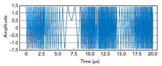
Figure 7 DDS output waveform with the typical LPI code.
IMAGE TEST RESULTS AND IMAGE QUALITY
aiRadar instruments provide ongoing image quality assessment tools to monitor performance by measuring quantitative performance parameters such as impulse response function, peak sidelobe ratio and ISLR.
Figure 8 is a screenshot from the aiRadar image quality analysis tool captured during preliminary calibration of the RRI-100 radar. It shows a point scatterer in a clutter rich short-range environment. Annotations on the image are added for clarity.
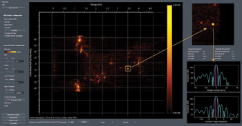
Figure 8 Screenshot from the image quality analysis tool.
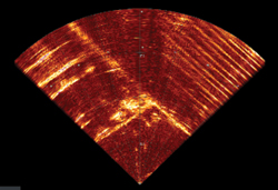
Figure 9 Image of parking lots and rail yards.
Figure 9 shows an image of two parking lots with vehicles, dumpsters and a railway switching yard. A relatively shorter range of 50 m is selected to demonstrate filtering and down-sampling of the 20,000 range samples at 5 cm resolution. The radar was deployed at an elevation of 20 m with the elevation boresight horizontal.
MTI
ADAS requires excellent MTI processing to separate stationary infrastructure, such as buildings and traffic signs, from moving or stationary objects, such as cars, trucks, cyclists and pedestrians. V- and W-Band provide excellent sensitivity and resolution of moving objects. A stationary radar image with normal processing is shown in Figure 10a, the outlined area expanded in Figure 10b. The expanded area processed with 32 chirps in a frame and reprocessed with a 32-bin Doppler filter (i.e., 32-point FFT) clearly shows the moving target (see Figure 10c), which was invisible in the normally processed image.
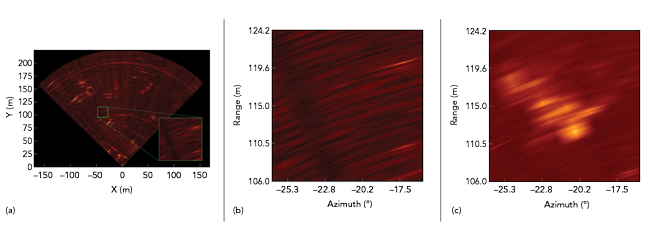
Figure 10 Stationary radar image with normal processing (a), expanded view of highlighted area (b) and highlighted area with MTI processing (c).
CONCLUSION
aiRadar research radars facilitate the definition of validated requirements and AESA configurations for emerging commercial, military and academic radar applications. These research instruments provide the tools to validate requirements and develop sophisticated radar systems reducing time-to-market and offering a low risk path to commercialization and deployment. aiRadar offers in-house radar design for a customized application-specific radar or licensing of the aiRadar programming language (aiRPL) compiler and the radar processing unit IP Core (aiRPU). Developing compact low size, weight, power and cost, AESA radars with RAR, SAR, InSAR, multi-baseline MTI, LPI and CA has never been easier.