
Spectrum analyzers have quickly evolved and made huge technological leaps from the initial instruments created in the 1960s, especially with the discovery of the fast Fourier transform (FFT); however, since most signals today are not continuous, but are modulated, some legacy measurement methods are simply not good enough and can lead to incorrect results.
Examination of a signal in the frequency domain is one of the most frequent tasks in radio communications, and such a task would be unimaginable without modern spectrum analyzers. Those instruments can analyze a wide range of frequencies and are irreplaceable in practically all applications of wireless and wired communications. With technological advancements, more is expected of spectrum analyzers, including the analysis of average noise levels, wider dynamic range and increased testing speed.
THE ORIGINAL SPECTRUM ANALYZER
Since the original spectrum analyzers were developed, the architecture has been based on an analog heterodyne receiver principle. The area circled in red in Figure 1 comprises real analog components. These components are responsible for rectifying the down-converted input RF signal to a video signal or voltage. The signal is further processed to determine how the result is displayed on the screen. A CRT type display in the early days allowed the user to view the measurements.
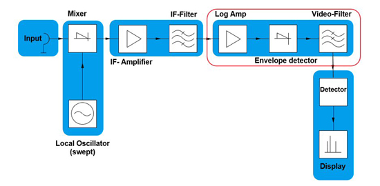
Figure 1 Original spectrum analyzer block diagram.
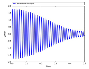
Figure 2 Modulated RF waveform.
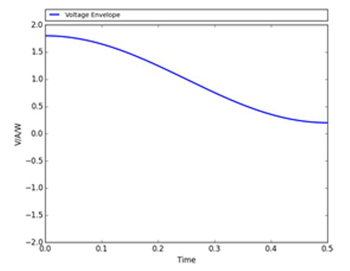
Figure 3 Rectified waveform.
The spectrum analyzer is only interested in the amplitude of signals in the frequency domain and in the early years, as now, people were mostly interested in the power of the spectral components. The envelope detector circuit converts the signal, either a continuous wave (CW) or modulated RF waveform (see Figure 2) and rectifies it, resulting in a video (envelope) voltage (see Figure 3).
Of course, the combination of a log amp and envelope detector is logarithmic in nature and, for that reason, early measurements with spectrum analyzers that dealt with power were always treated as logarithmic quantities. It is obvious that the unit of dBm is a logarithmic quantity, but the voltage data from the very first conversion starts as logarithmic; then, the data reduction that happens further in processing can cause some interesting effects.
RMS POWER AS THE TRUE POWER MEASUREMENT
In the past, power measurements were made using logarithmic detection. The peak detector was “calibrated” to show the correct level for CW tones and, in the early days, the measurement of CW signals was most likely sufficient. Using trace averaging reduces the level of noise shown on the trace. Because carrier power measurement - not noise power measurement - was the focus, engineers rarely converted values to linear quantities (e.g., watts) prior to performing averaging. Instead, the instrument performed trace averaging by simply averaging the dBm values.
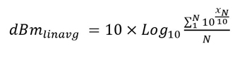
Using trace values represented as x in the equations below, the usual method employed in early analyzers was simply to sum up the logarithmic values and calculate the average:
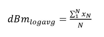
The correct way to do it is to convert the logarithmic values to linear values, calculate their linear average, then re-convert them to logarithmic values at the end:
Today, signals are not just CW but often incorporate some sort of modulation, so the method of measuring those signals correctly needs to change to measure the correct power level for both the carrier itself and its adjacent noise quantities. The notable standards setting organizations, such as the NPL (National Physical Laboratory) in the U.K., the PTB (Physikalisch-Technische Bundesanstalt) in Germany and NIST (National Institute of Standards and Technology) in the U.S., typically measure root mean square (RMS) power. From Ohm’s law, P = V2/R is the RMS power produced. This is accepted worldwide as the standard measure of power; it is fully defined and understood.
COMPARISON OF LOGARITHMIC AVERAGING VS. RMS TRUE POWER MEASUREMENTS
In early spectrum analyzers, the available detectors were typically peak, sample or minimumpeak, and these do not distinguish between linear or logarithmic values, since a peak is a peak (see Figure 4). There are three traces, each measuring a CW (no modulation) signal with a marker for each trace. In this case, all three markers measure the same power level of -0.3 dBm.
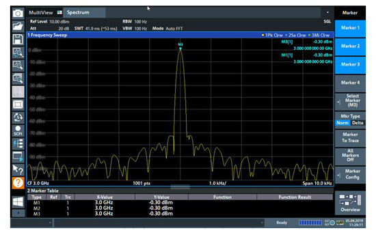
Figure 4 Display of power on an early spectrum analyzer.
This is fine for continuous waveforms, but what about modulated waveforms? Today, most signals are not CW but are modulated, and the user would benefit from using trace averaging to provide a smooth response with a high level of measurement repeatability (see Figure 5). Many signals designed to have modulation appear like Gaussian noise, so this example is highly relevant.
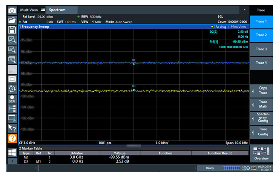
Figure 5 Modern spectrum analyzer display of a modulated RF waveform.