
Here, the typical detector used in legacy spectrum analysis is the sample detector, which always picks the Nth sample out of M samples taken within a timeframe T. If trace averaging is performed on this logarithmic data (trace 1) and compared to a true RMS measurement (trace 2), the result is 2.5 dB lower than the RMS power. This could cause serious problems for the user if wrong measurement settings are applied, or trace averaging is used with legacy trace modes or detectors that are logarithmic in nature.
WHAT IS LIMITING ACCURACY AND SPEED, EARLIER STANDARDS OR TEST DOCUMENTS?
During my career at Rohde & Schwarz, I have seen many tests from customers that were written using legacy equipment, though they were meant to be implemented using modern equipment. While it is entirely possibly to perform measurements as originally intended, this leads to two fundamental problems:
- The high risk of users doing manual measurements (e.g., those that are not led by test documents or specifications) with different results in linear and logarithmic calculations due to trace averaging, resulting in measurement errors.
- Users not using more accurate, automatic linear measurements with significantly improved speed and repeatability.
HOW DO MODERN INSTRUMENTS SOLVE THIS PROBLEM?
In a modern instrument, everything beyond the IF filter is digital (see Figure 6). Even the resolution bandwidth filter (RBW) is digital. Because of this, it is much easier to include different types of detectors with true linear power characteristics. Digital signal processing now handles many things, from the sharpness and fast settling time of filters to frequency response correction. Modern instruments also come with RMS detectors standard. This allows linear trace averaging if required, and there are other interesting effects of the RMS detector depending on the type of signal analyzed.
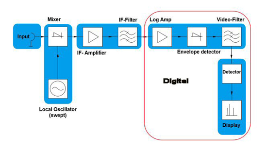
Figure 6 Modern spectrum analyzer block diagram.
Modulated Signals
As previously mentioned, the RMS detector yields a true power measurement. The sweep time, span, RBW and sweep points define the amount of averaging within a trace. Assuming the span, RBW and sweep points are fixed, one would typically increase the sweep time rather than averaging traces to get a more averaging effect. If an FFT mode is available, more samples can be captured for the same sweep time, which results in a higher amount of averaging and smoother traces. This is typically the best choice for averaging and is great for use with modulated signals.
Continuous Waveform Signals
Close attention must be paid to the span/RBW ratio and the number of sweep points. The RMS detector does not only average over time but also over frequency, so it is required to have at least one sweep point per RBW. Using a single point per RBW can lead to measurement errors and the signal power appearing lower than actual. A useful rule of thumb is “sweep points >5x span/RBW” to provide a correct power level.
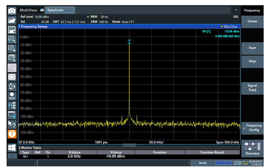
Figure 7a Signal source measured incorrectly with 1001 sweep points.
For example, Figure 7a uses an RMS detector with a CW signal over a span of 500 kHz and an RBW of 50 Hz. The output from the signal source connected to the spectrum analyzer is 0 dBm. In this case, the 5x span/RBW = 50,000, but the number of sweep points is set to 1001, and the result is a level displayed that is approximately 10 dB too low. If the number of sweep points is set to 50,001, in line with the requirements calculation, then the correct result of 0 dBm is obtained (see Figure 7b).
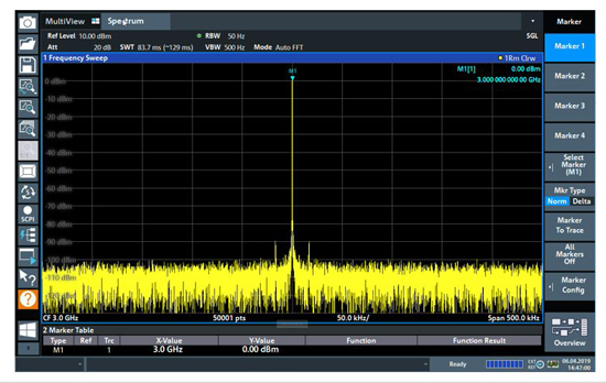
Figure 7b Signal source measured correctly with 50,001 sweep points.
Speed
The method of using an RMS detector with increased sweep time instead of utilizing trace averaging also produces significantly faster measurements, considering results with an equivalent standard deviation. For example, consider the power measurement of a modulated, noise-like signal with a repeatability of around 0.1 dB, using the settings in Table 1.
TABLE 1

To illustrate the statistical speed improvement, a test script can measure both the time taken to retrieve a measurement result and the result itself. Over many measurements, the standard deviation of the results is calculated. On a modern signal and spectrum analyzer, the results are summarized in Table 2. The standard deviation of measured amplitude is less than 0.1 dB (see Figure 8); and, more importantly, the time taken to do the test is greater than 5 times faster using the modern RMS detector method (see Figure 9). This is true even when the sweep time of test case 1 is just 0.01 that of test case 2.
TABLE 2
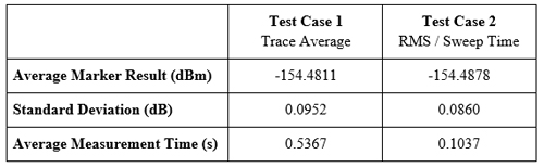
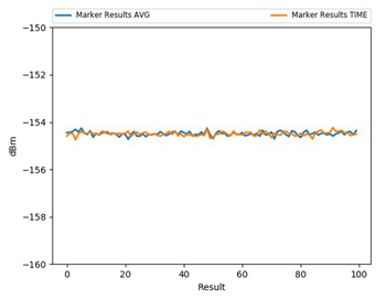
Figure 8 Comparison of measured amplitude for the trace average versus the RMS measurement method.
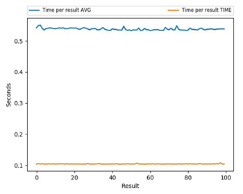
Figure 9 Comparison of measurement time for the trace average versus the RMS measurement method.
Running a similar set of tests with a varying sweep time, together with recording the time per measurement and the associated deviation in results, shows the improvement in test time (see Figure 10). Allowing the deviation in results to increase from 0.1 to 0.2 dB yields a further factor of 4x greater speed improvement, indicated by the red crosses on Figure 10.
Modern signal and spectrum analyzers are quite different instruments compared to those that existed 20 or so years ago. They incorporate a variety of measurement features that align with the accepted norms needed for industry today, while allowing measurements to be made using legacy methods. This can save significant time for engineers and increase measurement accuracy by using the newer incorporated features - only if engineers adopt new measurement methods versus those written in test or standards documentation from the last decades.
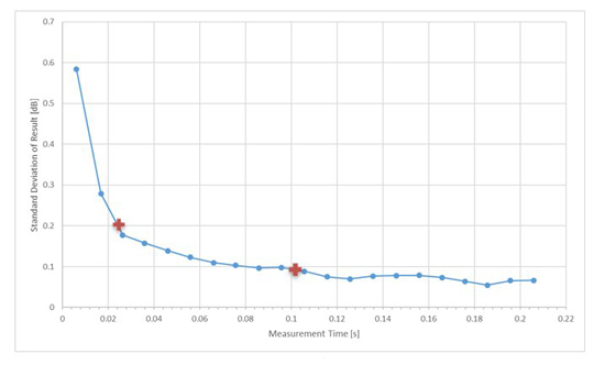
Figure 10 Standard deviation of measurement results as a function of measurement time for the RMS measurement method.