
Bit Error Rate (BER) remains the ultimate quality metric for all communication systems. Emerging 4G systems like LTE specify throughput rate as a metric for system performance. These 4G systems add intelligence by using adaptive modulation based on channel quality, but under the hood, BER is measured while the modulation is adjusted.
BER is measured by comparing the transmitted bit sequence to the received and recovered bit sequence. For a good comparison, the two sequences must be synchronized and aligned. Any slight misalignment—whether from the Device-Under-Test (DUT) or other parts of the simulation/measurement system—may lead to an erroneous BER. In a typical BER simulation/measurement system, comprising a signal generator, DUT and signal analyzer, the signal generator and analyzer may introduce amplitude, phase and time delay errors.
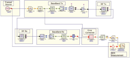
Figure 1 Shown here is an example of a complex communications measurement system.
With careful consideration and mathematical processing, these systematic errors can be removed. What’s required is a simple, systematic and automated method for calibrating the simulation/measurement system. We propose one approach. For the purposes of this article, it is implemented on the SystemVue simulation platform, although it is generic and can be employed using any simulation tool. This calibration method enables engineers to accurately simulate or make actual measurements on a DUT.
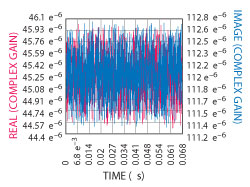
Figure 2 Errors in amplitude, phase and time delay in a practical measurement system can be quite complex and not something that can be calculated by hand.
BER Simulation
For simple measurement systems, amplitude errors, phase and time delay errors can be calculated by hand. For more practical systems, these errors are more complicated and can only be corrected algorithmically. Consider the complex system shown in Figure 1, which includes RF sections in the transmitter and receiver. A DUT (e.g., a communication channel) might also be included between the RF transmitter and receiver to determine its BER. Before doing that, however, it is necessary to ensure that the measurement system itself has a zero BER.
If a simulation is performed on the measurement system, alone, it may not have a zero BER because the baseband and RF filters introduce finite time delays. Additionally, nonlinear RF components exhibit AM-PM conversion in saturation giving rise to phase rotation. Moreover, RF components may have non-ideal amplitude and phase responses within the information bandwidth. These three error contributors—amplitude, phase and delay—must be corrected in the output bits before they are compared to the input bits in the BER sink. For example, the complex gain that must be applied to the symbols through the system shown in Figure 1 is displayed in Figure 2.
With a tool like SystemVue, engineers can write correction algorithms and turn them into custom models to aid in model-based engineering. To estimate these errors, the input bit sequence must be known. The input bit sequence may not be known, however, it may be randomly generated and encrypted. In order to perform the amplitude, phase and delay corrections, a known bit sequence is employed. This is generally referred to as framing the data by adding a preamble. The system in Figure 1 includes this framing concept and algorithmic components.
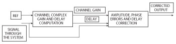
Figure 3 This correction algorithm can be used to correct for systematic errors.
After the bits go through the baseband transmitter, RF transmitter, RF receiver and baseband receiver, they may have undergone amplitude, phase and delay changes. This must be corrected before comparing them in the BER sink, a process that can be accomplished using the correction algorithm illustrated in Figure 3.
In a two-step process, this model (1) computes the amplitude, phase and delay errors and then (2) applies corrections on the framed input symbols, resulting in completely corrected and synchronized output symbols. The key is that known preamble bits are used in the computation of amplitude, phase and delay errors.
The pseudo-code for the algorithm’s amplitude and phase error correction is as follows:
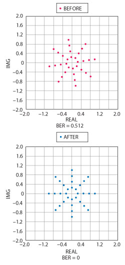
Figure 4 Shown here are two diagrams for user-defined constellations, illustrating the before and after effects of implementing synchronization algorithms.
-
Define Input ports as Input and Ref
Define Output port as Output
Assuming Sizes of Input signal, Reference signal and Output signal are the same. -
Get size of Reference signal
Ref_Size = Number of Ref signal points - Define and Initialize internal variables of Corre and Corre_1 for correlation results
-
Set Corre = Correlation (input, Ref)
Set Corre_1 = Correlation (Input, 1./Ref) -
Find Delay between Input and Ref
Abs_Corr = abs (Corr)
Delay_Index = find ( Abscorr == max(abscorr)) -
Find Channel Imbalance
Channel_Imbalance = Corr_1(Delay_Index)/Ref_Size - Output = Output/ Channel_Im balance
Assuming that the amplitude, phase and delay errors in the system are constant (i.e., systematic), then the above correction should result in a zero BER.
To illustrate the effectiveness of the synchronization algorithms, consider the simulation results in Figure 4. Here, the constellation diagrams before and after application of the synchronization algorithmic blocks are shown, along with the BER. The case represented in the diagrams is for a user-defined constellation, demonstrating the algorithm’s generality for any type of modulation format. Note that a delay correction alone will not synchronize the input and output bits – in this case, phase rotation is the cause for the high BER. The engineer may attempt to manually rotate the constellation using a phase shifter in the signal path, but the rotational symmetry of the constellation makes this tricky and tedious. The engineer may not know, for example, how many rotations the signal has undergone, making a stronger case for the algorithmic approach.
As can be seen from the constellation, there are a total of 32 points distributed as 4 amplitude states and 8 phase states. If these points are generated as complex numbers, they can then be specified as the mapping states in the Mapper and DeMapper components. Also, each symbol can be generated from five bits since log232 = 5. Hence, BitsPerSymbol = 5. The equations governing the generation of mapping states for a user-defined constellation are given by:
Amplitude_states=4
Phase_states=8
A=0.25
B=(pi/4)(0:Phase_states-1)
V=A(cos(B)+jsin(B))
MapperStates=[1pV 2pV 3pV 4pV]
Simulating BER oF A NOISY COMMUNICATIONS Channel/DUT
Once the system is calibrated, the BER of the DUT (in this case, a noisy communications channel) can be simulated. While doing this, the engineer should apply the amplitude, phase and delay corrections that are caused by the system only, and not by the channel. The implementation is shown in Figure 5.
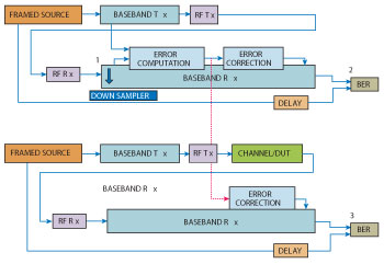
Figure 5 In this block diagram, measurement of a noisy communications channel is simulated. Only the amplitude, phase and delay corrections for errors caused by the measurement system are applied.
The output after the modulator in the baseband transmitter is split into two paths. One of the paths (the top one in the figure) goes through the baseband transmitter, RF transmitter, RF receiver, baseband receiver, and the algorithmic blocks to compute the measurement channel gain (which causes amplitude and phase errors) and sync index (which causes time delay). These errors are corrected.
The lower path, after the modulator in the baseband transmitter, goes through the noisy channel/DUT and then through the baseband receiver where it is corrected for channel gain and sync index errors computed in the other path. This corrects the systematic errors in the measurement system but does not affect errors introduced by the noisy channel/DUT. Finally, the BER computed at Location 3 in the figure reflects errors caused by the noisy channel/DUT only.
A few details must be noted while running the simulation represented in Figure 5. First, the engineer must adjust the phase of the down sampler at Location 1 in the top portion of the figure, so that the BER at Location 2 is reduced to zero. Second, the energy per bit/noise power spectral density ratio (Eb/N0) can be varied by setting the corresponding noise density in the noisy channel/DUT to simulate BER as a function of Eb/N0.
BER Measurement
Performing a BER measurement on an actual DUT is very similar to the simulation, although it is now a three step process.
(1) Download the Waveform to a Signal Source
A framed signal is created by adding a known preamble to the user data. Next, the signal is mapped and modulated with the required modulation format and then downloaded to a vector signal source. The downloaded waveform resides in the Random Access Memory (RAM) of the signal source. A digital vector signal source provides the functionality of digital up conversion and modulation onto an RF carrier.
(2) Calibrate the Measurement System
The signal generator’s output is connected to a signal analyzer through a low loss cable. The signal is received by the analyzer and may be captured in the form of I and Q files, which can then be run through the baseband receiver in the software. Typically, after the receive filter (a matched filter), the symbols are corrected for the amplitude and phase errors and also the time delay. The receive filter is usually a decimation filter. The phase of the decimation must be properly chosen to obtain good synchronization after error correction. The error computation and error correction follows the same method shown in Figure 3.
(3) Measure the BER of the DUT
In this step, the DUT is connected between the signal generator and the signal analyzer, making sure that the cable used in Step 2 is the only additional hardware besides the device. Any adapters used must be electrically small and should be low loss. Again, the signal is captured from the signal analyzer in the form of I and Q files for software processing. Baseband processing in software now needs to apply only the corrections determined in Step 2. The input symbols at the input and the output after error correction will not be perfectly synchronized if the DUT contributes a finite BER. The BER measurement then reveals only the BER of the DUT.
Conclusion
BER simulation and measurement of signals with common or proprietary modulation, coding and encryption can be difficult. One way to simplify this process is by following a systematic method that takes advantage of an algorithm to correct for measurement system amplitude and phase errors, as well as time delay. The measurement system calibration described here can be done automatically and adapts to any type of modulation format. For more information on this topic, go to http://cp.literature.agilent.com/litweb/pdf/5990-7757EN.pdf and http://edocs.soco.agilent.com/display/sv201301/SystemVue+E-Books+Gallery.