
 | |||
Demand for smaller, more densely packed and more powerful RF and microwave components is increasingly driving developments in a wide variety of areas, from chip packages to hand-held communication devices to phased-array antennas. In turn, the components and structures are experiencing increased levels of coupling between the electromagnetic fields and the thermal and structural effects, affecting their performance, durability and reliability.
Accordingly, the cross-coupling effects necessitate not only better electrical and RF design but also better integration with both mechanical and thermal design. Take a high power RF filter, for example. Its electromagnetic (EM) behavior will be determined by its materials, size, shape, and input frequency and amplitude. While simulating the filter in either a circuit or an EM simulator gives a good indication of its nominal circuit/EM behavior, the thermal and structural consequences of the EM fields are not readily visible.
In a real component, excessive heat can produce deformation that can de-tune the filter. Furthermore, while it is possible to drive a simulation of the filter with excessively high levels of simulated energy (with no apparent degradation of performance), in reality the filter would be destroyed.
Evaluating the thermal and stress aspects of a design typically falls to the thermal and mechanical engineers/specialists, respectively. However, these specialists seldom see the component design until it is passed ‘over the wall’ from the RF designer, by which time the RF engineer may have already done much work to optimize the design for performance.
If the thermal and/or stress analysis then finds that the device is likely to deform, or that it will require extensive cooling measures, then the aforementioned optimization may have been a wasted effort, as the RF engineer now needs to ‘have another go.’ This iterative passing to and fro is inefficient. However, the number of passes can be greatly reduced (and more confident) if the RF engineer performs thermal and stress evaluations during his component/structure design flow.
The ePhysics Solution
Ansoft’s ePhysics has been designed specifically to address this issue. With its coupled electromagnetic stress and thermal simulation capability, the tool is designed to enable electrical designers to perform complex and demanding multidisciplinary simulations.
In performing such evaluations, both steady state and transient thermal analyses are of interest, with the heat source of EM nature (power losses) ideally viewed over a broad range of frequencies. The power losses can occur on surfaces only, or on surfaces and within volumes depending on the electrical conductivities of the materials. Also, for completeness, the thermal analysis needs to include all three basic heat-transfer mechanisms — conduction, convection and radiation.
The first step towards visualizing the thermal characteristics of the design is to evaluate, with EM modeling software, the distribution of power losses in the component due to both surface and volume currents.
The next step is to map the power-loss density distribution from the finite-element mesh of the EM model to the finite-element mesh of the thermal model. Once the solution of the thermal problem is acquired, the RF engineer can inspect the overall temperature distribution and location of hot and cold spots for any instant in time.
Once calculated, the temperature distribution (of either static or transient thermal calculations) can be channeled into an elastostatic (structural stress) solver to evaluate the induced mechanical stress and to determine the deformation that will occur. In addition, the forces exerted by any low frequency EM fields can also be used in a separate model to analyze the corresponding stress.
Results include maximum principal stress, orientation of principal planes and the maximum von Mises (equivalent) stress. Here, the mechanical engineer may wish to state certain pre-handover stress criteria. Furthermore, once the electrical engineer has determined the deformations, he can close the loop and determine how these deformations affect the electrical performance of his design. How this can be done using ePhysics, in conjunction with Ansoft’s HFSS software, will now be explained.
Worked Example
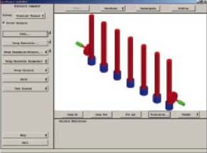
Figure 1 shows a seven-pole Chebychev filter, as might be used as a high power bandpass filter in the broadcast industry. Its physical dimensions are 280 by 30 by 120 mm and it comprises seven metal rods suspended from (and in electrical contact with) the ‘ceiling.’
 | ||
| Fig. 1 A seven-pole Chebychev design. | ||
The tips of the rods intrude into but do not contact with metal ‘buckets,’ which are in electrical contact with the ‘floor’ of the filter. There is approximately a 1 mm gap between each rod tip and its bucket’s wall. Each rod and bucket constitutes a resonator. The disks at each end of the filter are the coupling antennas and are primarily responsible for energy transfer into and out of the filter.
The filter was designed to have a bandwidth of 15 MHz, centered around 400 MHz. When simulated in Ansoft’s HFSS (v9.1) it can be seen that the design goals were attained (see Figure 2). The next step was to assess the filter’s thermal properties. The surface losses were exported from HFSS and imported into ePhysics. It was only necessary to export the surface power losses as the volumetric losses in air are negligible. It should be noted that if this example’s Chebychev filter were to be used with a heat sink (or were to be mounted on any other structure with a view to dissipating heat) it would have been at this stage that the heat sink or structure would have been imported from a mechanical CAD tool.
 | ||
| Fig. 2 The rise in the average temperature of the filter over a two hour period, as simulated in ePhysics. | ||
The mesh was exported from HFSS but only to support the information in the power loss file. The thermal solver made its own mesh. Next, in ePhysics, thermal and mechanical material properties were applied from a built-in database. For example, the aluminum used in the design was assigned:
- Thermal conductivity = 237.5 W/(mK)
- Mass density = 2,689 kg/m3
- Specific heat = 951 J/(kg K)
- Young’s modulus = 2.6e+10 N/m2
- Poisson’s ratio = 0.31
- Coefficient of thermal expansion = 2.33E-005 1/K
In addition, a boundary condition was set on the outer surfaces to represent the heat exchange between the device and its surroundings. Also, a boundary condition for the stress simulation constrained the ends of the filter to disallow any displacement.
Next, the transient thermal simulation was defined — minimum and maximum step size and total simulation time were set to 0.001, 500 and 7,200 seconds, respectively. As for the stress (deformation) analysis, the simulation engine was told to produce final figures only.
Figure 3 shows the average temperature rise over the simulation period (ending at about 76°C) and Figure 4 shows the components’ temperatures at the end of the simulation (with the temperature of the resonator poles rising as high as 80°C and antenna disks reaching 90°C).
 | ||
| Fig. 3 The rise in the average temperature of the filter over a two hour period, as simulated in ePhysics. | ||
 | ||
| Fig. 4 Hot spots in the filter at the end of the two hour simulation. | ||
Figure 5 shows the displacement, one of the most valuable outputs of the exercise. While the displacement shown is greatly exaggerated, it does demonstrate that the filter deforms — with the end faces constrained, the floor and ceilings bow out and the rods increase in length. Plus, the most dramatic effect is how the first and last rods bend inwards.
 | ||
| Fig. 5 Displacement (not to scale) at the end of the two hour simulation. | ||
The simulation revealed that the ceiling and floor are now 0.2 mm (average) further apart, the rods have increased in length by 0.15 mm (average) and the outer rods (which couple to the antennas) have tilted inwards by 0.07° or 0.14 mm.
Admittedly, these are not huge displacements, but it must be remembered that (because their RF characteristics are down to the physical dimensions and spacing of the rods) Chebychev filters are typically manufactured to a tolerance of 0.1 mm. In other words, many dimensional changes due to expansion have exceeded the manufacturing tolerances.
The detailed dimensional changes were used to update the geometry in HFSS to examine the filter’s new EM/RF performance, and the results can be seen in Figure 6 (which shows both new and old characteristics).
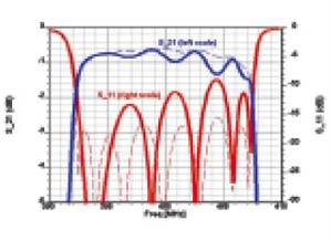 | ||
| Fig. 6 The filter’s new RF characteristics (solid lines) based on changes due to expansion and deformation, compared to the originalcharacteristics (dotted lines), as modeled in HFSS v9.1. | ||
In essence, the filter did not shift in frequency (still 400 MHz) and the bandwidth remained at 15 MHz. However, the ripple in the transmission is much more pronounced. The return loss has become worse — from –15 to –10 dB — and less symmetrical. Even though the filter still works, the deteriorations in the ripple and the return loss have become a cause for concern.
| |||
Other Applications
The bandpass filter is just one example of a wide variety of high power components where heating due to EM losses can be a problem. Another example is a ferrite circulator, where even modest heating can bring the ferrite above the Curie temperature and disable it.
A different class of applications is found when components are densely packed, and heat dissipation is a problem. Examples include chip packages and phased-array antennas. Another application is in chemical and industrial processes where microwave heating is intentional.
Finally, in the biomedical world, analyses of the effects of heating as a result of EM fields on tissue and bone will aid many biomedical applications, such as treating hyperthermia, and also further aid the study into the effects of using cell phones against the human head.
Conclusion
As the worked example demonstrated, exporting power losses from an EM simulation makes it possible for the RF engineer to conduct both thermal and stress analyses prior to handing the design over to thermal and mechanical specialists. Furthermore, as the thermal and stress intelligence was derived from the detailed EM characteristics, they are likely to be more accurate than analyses based on average losses. Finally, the EM characteristics are likely to change as the component/structure heats up, as was seen to be the case for the Chebychev filter.
Ansoft Corp.,
Pittsburgh, PA (412) 261-3200, e-mail: info@ansoft.com,
www.ansoft.com.