
Figure 1 Interference scenarios.
Autonomous driving is a current global trend that will continue to accelerate in the future. A key enabling technology in this area is automotive radar sensors, which are a significant step toward more driving comfort, crash prevention and even automated driving. Driver assistance systems are already common and many are supported by radar.
Today’s 24 GHz, 77 GHz and 79 GHz automotive radar sensors clearly need to be able to measure and resolve different objects while offering high range, radial velocity and azimuth resolution in any urban or rural environment. A very important feature is immunity to interference from other automotive radar sensors. This topic has not been greatly focused on since the market adoption of radar sensors is low at the present time. However, the proliferation and expected growth is continually increasing and the Advanced Driver Assistance Systems (ADAS) market is expected to grow by up to 10 percent per year.
Considering that 72 million new cars are registered each year with a potential average of three (or more) automotive radar sensors per car, about 200 million more automotive radar sensors could be on the streets in the not too distant future. Consequently, the 24 GHz and 76 to 81 GHz spectrum will be heavily occupied. Automotive radar sensors will need to cope with mutual interference and offer signal diversity and interference mitigation techniques.
Figure 2 LFMCW radar signal with upchirp and downchirp.
The occasional accidents involving automated cars that are under research and development have been reported in the press. In May 2016, questions about the security of self-driving cars and the safety of the technologies rose again after the first fatal accident involving a partially automated car. It is therefore essential to ensure the functionality of the sensing equipment in any environment in the presence of mutual interference.
This article presents the theoretical background of state-of-the-art and next generation automotive radar signals and sensors. It explains the impact of mutual interference and presents measurement possibilities to test and verify mitigation techniques in arbitrary RF environments with norm interferers. This approach helps researchers and developers engineer automotive radar sensors that function according to specification, even in harsh RF environments.
Figure 3 Chirp sequence.
AUTOMOTIVE RADAR AND REGULATIONS
Several automotive radar sensors may interfere with each other when operating in the same portion of the frequency band1 and in close proximity to each other (see Figure 1). Possible scenarios are the creation of artificial ghost targets or decreased probability of detection. Ghost targets do not exist in reality, but appear as real targets to the radar sensor. This may be caused by a copy of the transmitted signal. The copy is not from the original radar transmitter, but falls into the receiver bandwidth and is processed as a real echo signal. For this scenario to occur, timing, waveform and frequency between two or more radars have to match and the echo power has to exceed a certain limit.
Also, arbitrary RF signals with a certain power level that fall into the receiver bandwidth may increase the noise floor of the radar and reduce the Signal-to-Noise Ratio (SNR) of a target. This may cause targets with a small Radar Cross Section (RCS) to disappear since the SNR of these echoes is reduced. For this scenario to happen, a signal that spreads over all frequencies after FFT signal processing has to fall within the receiver bandwidth.
The output power of automotive radar sensors is specified by the Electronic Communications Committee (ECC). Based on the ECC Decision (04) 03 entitled, “The Frequency Band 77 to 81 GHz to be Designated for the Use of Automotive Short Range Radars,” the European Conference of Postal and Telecommunications Administrations (CEPT) designated the 79 GHz frequency range for Short Range Radar (SRR) equipment on a non-interference and non-protected basis. Moreover, a maximum mean power density of -3 dBm/MHz e.i.r.p. associated with a peak limit of 55 dBm e.i.r.p was defined, and the maximum mean power density outside a vehicle resulting from the operation of one SRR equipment shall not exceed –9 dBm/MHz e.i.r.p.
All standard automotive radar sensors operating in these bands have to fulfill this criteria. ETSI standards EN 301 091-1 and EN 301 091-22 already standardize several aspects related to test conditions, power emission and spurious emissions for 77 GHz radars, but do not mention anything about interference rejection. The same is true for the ETSI standards EN 302 264-1 and EN 302 264-23, which regulate the 79 GHz band.
In the maritime domain, for example, navigational radars have to adhere to the International Electrotechnical Commission standard IEC 62388,4 which specifies the minimum operational and performance requirements, methods of testing and required test results conforming to performance standards of radiocommunications equipment and systems. One very important aspect in the IEC standard is the specification of interference rejection. However, for automotive radar specifications, there is no standard defining interference rejection or performance and test methods that navigational radars have been subject to for decades.
WAVEFORMS AND IMPACT OF INTERFERENCE
If an interfering signal falls into the radar receiver bandwidth, it should be detected as such and rejected in the signal processing. It is common for manufacturers to each have slightly different waveforms, timings, bandwidths, antenna patterns and signal processing. This is an advantage in terms of interference rejection, but also results in the radar responding differently to interference.
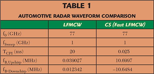
Figure 4 Effect of interference signals.
There are mainly two different types of waveforms used in today’s automotive radar sensors. Blind Spot Detection (BSD) radars often use the Multi-Frequency Shift Keying (MFSK) radar signal and operate mainly in the 24 GHz band. Radars operating in the 77 GHz or 79 GHz band often make use of Linear Frequency Modulated Continuous Wave (LFMCW) signals or Chirp Sequence (CS) signals, which are a special form of LFMCW signals. Using LFMCW, the radar transmits a frequency modulated signal (chirp) with a specific bandwidth fsweep within a certain time, called the coherent processing interval TCPI, as shown in Figure 2.
The radar down-converts the received signal with the instantaneous transmit frequency and measures the beat frequency fB, which describes the offset from the original transmitted waveform. Both radar parameters, range, R and radial velocity, vr, contribute to the measured beat frequency. In order to resolve the target unambiguously for vr and R, two beat frequency measurements are necessary (see Figure 2, where the beat frequencies are denoted as fB1, fB2). In multitarget situations, range and radial velocity cannot be resolved unambiguously by two consecutive chirps measuring different beat frequencies. This can be resolved by an additional chirp with a different slope.
To enable a certain radial velocity resolution, TCPI is typically in the region of 20 ms and the number of chirps for a single processing interval is greater than two. fsweep defines the range resolution and varies between 100 MHz and above, and will be more than 1 GHz in the near future and probably 4 GHz or even 5 GHz in the distant future.
The chirp sequence waveform consists of several very short LFMCW chirps, each with a duration of TChirp, transmitted in a block of length TCPI (see Figure 3). Since a single chirp is very short, the beat frequency is mainly influenced by the signal propagation time and the Doppler frequency shift, fD can be neglected.
Signal processing takes place following an initial down-conversion by the instantaneous carrier frequency and a Fourier transformation of each single chirp. Due to the high carrier frequency and the high chirp rate the beat frequency is mainly determined by range. The target range is calculated assuming a radial velocity,  . The radial velocity is not measured during a single chirp, but instead over the block on consecutive chirps with duration TCPI. A second Fourier transformation is performed along the time axis, which results in the Doppler frequency shift. After obtaining the Doppler frequency shift, the target range is corrected.
While a single TChirp is typically in the region of 10 µs to 100 µs, the number of signals LN should be so high that the entire coherent processing interval, TCPI=LN TChirp is again in the region of several dozen ms to achieve the desired radial velocity resolution.
The signal bandwidth is high, and the receiver bandwidth is very small in comparison. This can be achieved due to the fact that only the maximum beat frequencies for which the radar is designed are measured. To give two examples, Table 1 shows the resulting beat frequencies of two automotive radar waveforms when measuring a target in 40 m range with a radial velocity of 50 m/s.
These calculations are according to the LFMCW equations and show that the occurring beat frequencies are in the range of 100 kHz for LFMCW, but are much higher for CS radars (several MHz). This causes the receiver bandwidth to be higher and may require different mitigation techniques compared to techniques applied when using LFMCW.
Figure 5 Typical CW radar signals.
The advantage of CS compared to LFMCW is the unambiguity and the increased update rate, because a single coherent processing interval is sufficient to measure and resolve all targets in the observation range. In LFMCW, at least three different chirp signals are necessary. On the other hand, in the CS waveform the processing complexity increases due to multiple FFTs and the receiver bandwidth scales according to the expected beat frequencies, which is why there is a need for interference rejection and mitigation techniques.
Figure 4 depicts the down-conversion and Fourier transformation process when an interference signal (red chirp) is present. The interfering chirp is down-converted together with the radar return of the object. In green is the constant beat frequency for a certain range as it would occur in an interference-free environment while measuring a single target. With the introduction of an interference signal, a time-dependent beat frequency is generated (red curve), which appears in addition to the wanted echo. Hence in the Fourier domain, the spectrum shows not only a single beat frequency but several frequencies.
In the optimal solution, the signal-to-noise ratio of the echo signal (green bar) is maximum. When the interference signal is present, the noise floor rises and the signal-to-noise ratio decreases depending on the receiver bandwidth, fLP as indicated in the sketch. Aside from a decreased probability of detection, the lower signal-to-noise of an echo signal results in a less accurate range and a less accurate Doppler measurement.
The receiver noise floor and the signal-to-noise ratio of the object depend on the hardware, software and the object’s RCS. Typical noise floor levels are about –90 dBm for an automotive radar operating at 77 GHz. One trend is to combine chirp sequence waveforms with other methods such as frequency shift keying in order to reduce the computational effort. However, at present, there are no common definitions on normative interferers and interference rejection written in standards for automotive radar sensors.
T&M INTERFERENCE REJECTION
In order to verify the performance of interference rejection methods and to test the interference robustness of a radar sensor, a measurement was set up in the laboratory that allowed the generation of arbitrary RF signals. These signals can even include, for example, transmitter position, antenna motion and pattern.
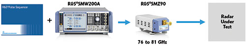
Figure 6 Interference test setup using a vector signal generator and multiplier.
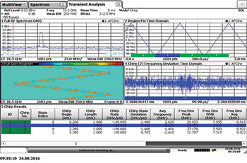
Figure 7 Radar interference signal.
Figure 5 shows typical radar interference signals generated by Pulse Sequencer software, such as LFMCW, frequency shift keying and chirp sequence. It should be mentioned that the software is not limited to these signals or sequences, but can also create complex RF environments to the laboratory.5
Although these signals can be generated in the baseband, bringing these signals up to E-Band frequencies is a challenge. As most automotive radars use only frequency-modulated signals, one way is to use a state-of-the-art vector signal generator together with a multiplier. The advantages of this setup are less complex test setups and high signal bandwidth that can be reached more easily since the multiplier also scales the signal bandwidth.6 The scaling factor can easily be considered when designing the waveforms in the baseband.
Figure 6 shows a typical test setup for automotive radar sensors, using a vector signal generator in combination with a multiplier. The Pulse Sequencer software is used to generate the arbitrary RF environment in which signals are transferred to the vector signal generator over the local network or via a USB stick. The RF signals produced by the vector signal generator at 12.6 to 13.5 GHz are multiplied by a factor of six. An E-Band horn antenna can be connected to the output of the multiplier so that the E-Band signal can then be transmitted over the air towards the Device Under Test (DUT).
In this setup, the bandwidth applied at the vector signal generator also scales by a factor of six. To generate radar chirps with a signal bandwidth of 5 GHz, a baseband bandwidth of 833.3 MHz is required (833.3 MHz × 6 = 5 GHz). With the setup shown in Figure 6, a baseband bandwidth of 2 GHz is possible, which results in an RF signal bandwidth of up to 12 GHz (2 GHz × 6 = 12 GHz).
Figure 8 Interference test setup using a mixer.
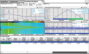
Figure 9 Radar sensor analyzed with the transient analysis option.
The spectrum of the interference signal is in Figure 7. It is possible to observe the spectrum and the LFMCW signals with upchirps and downchirps. All chirp signal parameters have been analyzed directly with a signal analyzer equipped with transient analysis software. The chirp length is 1 ms and the signal frequency linearity is in the domain of several kHz, which is comparable to automotive radar sensor signals.
Researchers have already investigated using communications signals like OFDM in automotive radar7 and designed interference rejection algorithms.8 However, it may be complicated to process these extremely wideband OFDM signals in a price-sensitive sensor in real time. This will make it complicated to apply OFDM signals in the near future. This is also one of the reasons why it is so important to verify interference rejection algorithms, waveforms and the entire processing chain, starting with the mmWave region.
Not only is the cost-effective, real-time processing of very wideband OFDM signals challenging, generating amplitude-modulated interference signals in mmWave also requires a more complex setup. One approach is depicted in Figure 8, which shows the IF and LO signals generated by a two RF channel vector signal generator. The LO signal is multiplied by a factor of six and shifts the IF signal to 76 to 81 GHz. A vector signal generator with an internal wideband baseband then allows the generation of arbitrarily modulated RF signals in the E-Band with a signal bandwidth of up to 2 GHz. Using vector signal generators incorporating calibrated internal wideband baseband hardware has benefits over solutions using multiple instruments since there is no need for calibration nor compensation of the I/Q frequency modulator response.
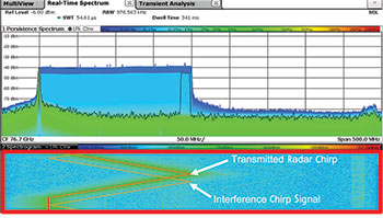
Figure 10 Real-time spectrum showing wanted signal (on left with single chirp) and continuously chirping interferer.
MEASUREMENT RESULTS
To verify the impact of additional radar signals that are present, a state-of-the-art 77 GHz sensor was used. The advantage of this sensor is the availability of IF and FFT raw data. This makes it possible to immediately verify the impact of interference signals on the FFT spectrum. As explained, one should see an increase in the noise floor depending on how much interference signal power is downconverted and falls into the receiver bandwidth. In these measurements, the sensor was configured to transmit an LFMCW signal with 200 MHz signal bandwidth as depicted in Figure 9, where the transient analysis option shows the duration, signal bandwidth, the linearity (frequency deviation time domain) of the transmitted chirps and spurious emissions in the RF spectrum.
The Pulse Sequencer software was used to emulate the waveform and test the radar with an additional interference waveform. The real-time spectrum in persistence mode can be used to verify the two signals. Figure 10 shows two RF signals, the chirp which is transmitted by the radar sensor and the interference signal generated by the vector signal generator. While the radar sensor transmitted an upchirp and downchirp followed by an unmodulated CW signal, the interference signals just transmit upchirps and downchirps. The power level of the interfering chirp is about 5 dB less than the transmitted radar signal as shown in the persistence spectrum.
Figure 11 depicts a sample of spectrum measurements where the amplitude level over the range is plotted with and without interfering signals present. While measuring into free space without interference, this radar sensor measures a spectrum at a power level in the range of -115 dBm and some radar echo signals in close range.
When an interfering signal is present, the noise floor increases to about -102 and -90 dBm depending on the interfering signal itself. It should be mentioned that this radar sensor does not apply any interference cancellation. Also, the noise floor increase strongly depends on the interference signal level and the interfering waveform itself as can be seen in the measurements. A decrease of 10 to 25 dB SNR has been proved, which can cause objects to be very easily lost during tracking or objects with low RCS, like pedestrians, going undetected.
Figure 11 Radar sensor spectrum.
Conclusion
Automotive radar supports the trend towards additional driving comfort, safety and even automated driving. The number of automotive radar sensors on the streets is increasing rapidly and will grow further in coming years. As a consequence, the allocated spectrum in the 24 GHz, 77 GHz and 79 GHz bands needs to be shared among different types of sensors and signals. As a safety critical element, the radar sensor needs to cope with mutual interference, offer signal diversity and interference mitigation techniques to measure, detect, resolve and classify radar echo signals even in the highly occupied frequency spectrum. Regulations and standards on interference test and mitigation are available for navigational radars, for example, but are not yet required for automotive radars.
To address these needs, this article explained the theoretical background and impact of interference on state-of-the-art and next generation automotive radar. Test and measurement possibilities to verify interference mitigation techniques in arbitrary RF environments have been presented. The impact of interference has been verified using a state-of-the-art commercial 77 GHz radar sensor. These test setups should help researchers and developers ensure the functionality of their radar according to specification even in harsh RF environments.
References
- MOSARIM Project, “D2.2 – Generation of an Interference Susceptibility Model for the Different Radar Principles,” 28.02.2011, www.transport-research.info/project/more-safety-all-radar-interference-mitigation, July 8, 2016.
- European Standard EN 301 091, “Electromagnetic Compatibility and Radio Spectrum Matters” (ERM); “Road Transport and Traffic Telematics” (RTTT); “Technical Characteristics and Test Methods for Radar Equipment Operating in the 76 GHz to 77 GHz Band,” www.etsi.org, July 8, 2016.
- European Standard EN 302 264, “Electromagnetic Compatibility and Radio Spectrum Matters” (ERM); “Short Range Devices;” “Road Transport and Traffic Telematics” (RTTT); “Short Range Radar Equipment Operating in the 77 GHz to 81 GHz Band;” “Part 2: Harmonized EN Covering the Essential Requirements of Article 3.2 of the R&TTE Directive,” retrieved from www.etsi.org, July 8, 2016.
- International Standard IEC 62388:2013, “Maritime Navigation and Radiocommunication Equipment and Systems – Shipborne Radar – Performance Requirements, Methods of Testing and Required Test Results,” Ed. 2.0, 2013-06-26.
- Rohde & Schwarz, “1MA267: Automotive Radar Sensors – RF Signal Analysis and Inference Tests,” Application Note, www.rohde-schwarz.com/appnote/1ma267, July 8, 2016.
- Rohde & Schwarz, “Pulse Sequencer Software,” www.rohde-schwarz.com/us/software/smw200a/.
- M. Braun, “OFDM Radar Algorithms in Mobile Communication Networks,” Dissertation, Institut für Nachrichtentechnik, Karlsruher Instituts für Technologie, Karlsruhe,” 2014.
- MOSARIM Project Final Report, 2012-12-21, http://cordis.europa.eu/docs/projects/cnect/1/248231/080/deliverables/001-D611finalreportfinal.pdf, July 8, 2016.