This is the second part of a three part post describing the architecture differences of spectrum analyzers.  In this post, I will breakdown the architecture different between the different types of Stepped Spectrum Analyzers and introduce some additional figures of merit.

Previously, I have focused on the swept architecture and introduced the first two figures of merit, speed and dynamic range.

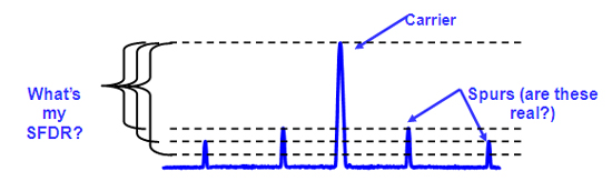
Figure 1 – Spur Free Dynamic Range is the best figure of merit to quantify dynamic range.

While discussing the maximum observable instantaneous bandwidth of a signal with the swept analyzer, I pointed out that the limitation is the maximum resolution bandwidth filter (RBW) of the analyzer.  Now with the stepped architecture, we get a hint at the next figure of merit.

Stepped Spectrum Analyzer - Vector Signal Analyzers

Analyzing pulsed signals or broadband signals carrying digital modulation requires vectormeasurements that provide both magnitude and phaseinformation. A simplified vector signal analyzer (VSA) digitizes all of the RF power within the passbandof the instrument and puts the digitized waveform intomemory.  The capture bandwidth can be up to the bandwidth of the last IF stage of the spectrum analyzer as long as the digitizer is sampling fast enough to meet the Nyquist criteria of the signal of interest.  The RBW no longer limits the power of the signal that can be seen, but now be used to improve the resolvable signals that can be seen within the passband.  This gives rise to the third important specification in the selection of a spectrum analyzer:  bandwidth.

The waveform in memory contains both themagnitude and phase information which can be used byDSP for demodulation, measurements or display processing.Within the VSA, an ADC digitizes the wideband IF signal, andthe downconversion, filtering, and detection are performednumerically. Transformation from time domain to frequencydomain is done using FFT algorithms. The VSA measuresmodulation parameters such as FM deviation, Code DomainPower, and Error Vector Magnitude (EVM and constellationdiagrams). It also provides other displays such as channelpower, power versus time, and spectrograms.While the VSA has added the ability to store waveforms

in memory, it is limited in its ability to analyze transientevents. In the typical VSA free run mode, signals that are acquired must be stored in memory before beingprocessed. The serial nature of this batch processingmeans that the instrument is effectively blind to eventsthat occur between acquisitions. Single or infrequentevents cannot be discovered reliably. Triggering on thesetypes of rare events can be used to isolate these events

in memory. Unfortunately, if the VSA has limited triggeringcapabilities, like they most often do, it is difficult to isolate a signal of interest.  Most VSA’s only have external triggering and IF level triggering capability.

External triggering requires prior knowledgeof the event in question which may not be practical. IFlevel triggering requires a measurable change in the totalIF power and cannot isolate weak signals in the presenceof larger ones or when the signals change in frequencybut not amplitude. Both cases occur frequently in today’sdynamic RF environment.

Another important attribute to consider on the signal processing on a VSA, is the amount of observation time required to render an FFT and the time between each FFT rendering.  If you assume a fixed FFT length, the observation time, or spectrum time, can directly calculated from the Window Function divided by the resolution bandwidth.

Spectrum Time = Window Factor/Resolution BW

Example: 

RBW = 300kHz;
Window Factor for Kaiser window = 2.23
Spectrum Time = 7.4 us

If the display is updated 10 times a second, only 74 us of signal are being observed every second.  The observation time is only 0.0074% of the time.  Or, to hint at the fourth figure of merit, minimum event duration for 100%probability of intercept, the signal can’t change between acquisitions to have 100% certainty you are not missing something with the signal.  This means that at an update rate of 10 times a second, the signal can’t change faster than every 100 milliseconds.

Real-Time Spectrum Analyzers

The term “real-time” is derived from early work on digitalsimulations of physical systems. A digital system simulationis said to operate in real-time if its operating speed matchesthat of the real system which it is simulating.

To analyze signals in real-time means that the analysisoperations must be performed fast enough to accuratelyprocess all signal components in the frequency band ofinterest. This definition implies that we must:

• Sample the input signal fast enough to satisfy Nyquistcriteria. This means that the sampling frequency mustexceed twice the bandwidth of interest.
• Perform all computations continuously and fast enoughsuch that the output of the analysis keeps up with thechanges in the input signal.

The figure of merit for minimum event duration for 100% probability of intercept has been to define minimum duration for observing a squarewave pulsed signal with 100% certainty at the absolute power level of the signal.  Real-time analyzers have a minimum event duration for 100% probability intercept figure of merit usually measured in low microseconds to 10’s of microseconds depending on resolution bandwidth setting.

Figures of Merit

So now that we have described the architectures, we have the ability to establish a new figure of merit to consider when selecting a spectrum analyzer:speed, dynamic range, bandwidth, and minimum event duration for 100% probability of intercept.

In the next entry, we are going to look at the observable differences in a signal using the three different architectures.