
The most common coaxial connector in the microwave market, the Sub-Miniature A connector (SMA), was first introduced by Bendix Corp. in the late 1950s as a connector specially designed for the 0.141" diameter semi-rigid cable. At the SMA connector’s inception, the operating frequency did not exceed 12 GHz.
As the design matured, the maximum operating frequency was pushed up to 18 GHz and eventually higher. Some years later, higher frequency connector interfaces were introduced with SMA compatible airlines, two examples being the 3.5 mm and 2.9 mm interface connectors. In various applications, the 3.5 mm interface is used to transmit signals at a frequency as high as 36 GHz and the 2.9 mm (SMK) interface as high as 46 GHz.
The theoretical limit of the operating frequency of the SMA connector is restricted by a second mode resonance. The connector will operate at higher frequencies than that of the second mode resonance; however, this would be a dual-mode operation transmission. This is undesirable for most applications, especially in high power applications, where second mode resonances will overheat the SMA connector and cause a voltage breakdown. Theoretically, the second mode can be excited from the so-called cut-off frequency, which depends on the transverse dimensions of the line and the effective dielectric constant. The first waveguide mode in a coaxial line is a magnetic mode, which is identified by TE11 or H11. In this article, either name will be used. The approximate cut-off frequency (in GHz) in a circular coaxial line is given by

where
d = center conductor diameter in inches
D = dielectric diameter in inches
ε = relative dielectric constant
the “cut-off frequency” Fc can be calculated with an uncertainty of five percent. If a better accuracy is needed, the equation given by Marcuvitz1 can be used. Note that the mode resonance will typically appear at a frequency greater than that of the cut off. Typical connectors require different sizes of coaxial lines behind the established interface area dimensions to accommodate various sizes of coaxial cable. The exact value of the resonance frequency for a connector depends highly on the length of the coaxial line with the lowest “cut-off frequency.” The shorter the length of this limiting coaxial line, the higher the resonance frequency and the higher the connector operating frequency.

This point, while straightforward, has a significant impact on the design and verification of the maximum operating frequency of a connector. When verifying the maximum operating frequency of a connector using a vector network analyzer (VNA), there are cases where the resonance frequency is not clearly visible. However, just because a component does not show a resonance on the VNA, it does not guarantee that there will not be any resonance in actual applications. The SMA connector is an excellent example of this phenomenon. The VNA test port connector has an airline interface (typically 3.5 mm). A 3.5 mm airline interface has a cut-off frequency of approximately 38 GHz, which is much higher than the SMA connector (approximately 25 GHz). While the 3.5 mm connector has an excellent electrical performance, its high cost limits its range of applications outside the test lab.
This is significant as it means that in a real application (see Figure 1), the SMA connector will be connected to another SMA interface.
Thus, the Teflon dielectric line length, the limiting coaxial line in this case, will be substantially increased as compared to the test situation.
The 3.5 mm interface airline can artificially increase the dielectric bead length because the airline has an inductive impedance for the TE11 mode below the cut-off frequency2,3 (see calculations in the Appendix).
However, the airline influence is much smaller when compared to the SMA Teflon line. In this case, the resonance frequency will be lower and its effects easily discerned. Computer simulations were performed for different resonance structures using HFSS from Ansoft.

Figure 2 shows a typical simulation of the second mode resonance performed by HFSS for the standard SMA line size with a contact diameter 0.050" and a Teflon diameter of 0.1625". There are several approaches that can be taken to create this resonance frequency simulation. Multiple modeling approaches were used and it was found that there were differences of several percent in the location of the resonance frequency. However, one model in particular proved to be the most repeatable, both in the simulation and the actual performance of the SMA connector while under test. This model was based on a homogeneous dielectric line with three modes on the ports. The blue line in Figure 3 depicts the results of the simulation of the resonance frequency versus the dielectric length of a SMA connector line connected between two 3.5 mm airlines. Note that the Y-axis shows the peak values of the resonance frequency. The maximum operating frequency of the connector must always be lower than the beginning of the resonance.
Various SMA components were tested and it was found that the second mode resonance was not always visible even under conditions where it was calculated to occur. Typically, the third and higher modes are much sharper and more discernable. This was the case when testing a SMA plug-to-plug adaptor, where the third mode resonance frequency was clearly visible while the second mode resonance was not. Based on the above formulae and the calculations based upon the length of the Teflon dielectric line, the adaptor should show a second mode resonance at approximately 26 GHz. However, this was not the case. Using several different calibrations and test methods, including special methods for the second mode detection described by the IEC 61141 report,4 as an Automatic Reflection Measurement Technique, there was still no success in identifying the second mode resonance frequency. The fact that this resonance is not always visible is well known.5 It is shown that the resonance was unnoticed until provoked by a special exciter. Apparently, under some conditions, the resonance magnitude is so small that it becomes negligible and the resonance issue can be ignored. In cases such as this, it is possible to produce a coaxial component based on a dielectric line of substantial length, which can be used for a single mode transmission at frequencies much higher than the cut off. Is this applicable for RF connector manufacturing? No. In real world applications, the mating connector geometry cannot be predicted. This is an important consideration as the mating connector’s dielectric length has a critical influence on the resonance magnitude. In addition to computer simulation and testing, it is always possible to perform some calculations. Typically, these calculations have some uncertainty in predicting the actual performance of the component. James Kubota noticed that when comparing calculated and measured results, the “relationship yields an approximate value that is lower than the exact frequency by a few percent.”5 When measuring and verifying the second mode resonance frequency, most references calculate the resonance frequency based on the conjugate impedance, using transmission line equations. However, a simpler method to compute the resonance frequency could be to use a waveguide resonance cavity approach.
The Teflon insulator, or bead, is actually an electrically short piece of a coaxial waveguide. Thus, the bead can be represented as a TE11 mode coaxial resonator filled with dielectric. It can be assumed that the connector resonance is related to the cavity resonator. The simple approach to calculate a resonance bead is through the minimum length of a coaxial resonator. According to references, the waveguide or cavity resonator is a piece of waveguide with a height equal to a half-wavelength. The cavity can be based on a circular or rectangular waveguide as well as a coaxial line. In this particular case, the Teflon bead is a coaxial line but with a waveguide mode. This means that the wavelength in the waveguide cavity is greater than in free space. There is an infinite number of resonant modes that may exist in this structure. The lowest mode, TE111, is of interest. The third unit in the mode designation means that one half-wavelength has to be in an axial direction. Thus, the length of the Teflon bead has to reach one half of the wavelength in a coaxial waveguide for TE11 mode. The wavelength in the waveguide filled with dielectric (λg) can be calculated from

where
λ = wavelength in free space, which is actually the TEM wavelength in the coaxial airline
λc = cut-off wavelength for the coaxial airline
εr = relative dielectric constant of the PTFE bead
The resonance length (l) is a half-wavelength, thus is equal to

In the case of the SMA connector, the standard SMA line is a PTFE-loaded coaxial line with conductor diameters of 0.050" and 0.1625" and a dielectric constant of approximately 2.03. The cut-off frequency of this line will be approximately 24.82 GHz. To calculate the minimum length of line that can excite resonance at a frequency of 27 GHz, the following parameters need to be calculated:
λ = 1.11 cm at 27 GHz
λc = 0.848 cm at 35.36 GHz. (The ‘cut-off frequency’ of a 0.050/0.1625" coaxial air line without dielectric.)
Introducing these values into Equation 2, the waveguide length λg for the TE11 mode will be 1.98 cm. The TE111 mode resonance is possible at half of the wavelength, which is 0.99 cm or 0.390". This means that an SMA connector junction with an overall Teflon dielectric line length of 0.390” for the mated pair is susceptible to resonance at a frequency equal to or greater than 27 GHz. Note that, if the frequency is gradually reduced to approach the cut-off value for the dielectric loaded line (24.82 GHz in this case), the resonance length will grow and it will approach infinity. This example explains why a component will never resonate at its cut-off frequency. The resonance frequency must be higher than the cut off, otherwise the bead length would be infinite.
Calculations based on Equation 3 closely match the HFSS data and the measured data until the Teflon is shorter than 0.250". At this point, there is a need for additional correction factors for shorter dielectrics. One reason is that the airline, connected to the Teflon bead, creates an inductive impedance at the frequency of interest for TE11.2,6 In the case of a Teflon dielectric line being connected to a coaxial airline, the effective dielectric length will be increased at both sides of the bead. This means that the physical length of the dielectric needs to be reduced to compensate for the increase in effective length. This length differential for each side of the bead can be approximately calculated as

(See Equation 9a in the Appendix.)
Here fc is the cut-off frequency of the connected airline (in this case a 3.5 mm airline) and fct is the cut-off frequency of the dielectric bead. If there are identical coaxial airlines connected to each side of the Teflon bead, it will be necessary to use twice the value from Equation 4. Another correction factor is caused by the junction between Teflon/airline or Teflon/Teflon. According to references, any such junction has a capacitive impedance. This capacitive impedance is typically compensated by an inductive step of a certain length (see, for example, area “b” on the SMA-to-SMA connection). Additionally, there are air gaps in the Teflon at the reference plane between the mating connectors (see area “a” on the SMA-to-SMA connection). Apparently, these steps push the resonance frequency up, so they have an opposite influence when compared to the length calculated from Equation 4.
The standard SMA line with a length of 0.390", when connected to 3.5 mm airlines at both ends, is susceptible to a mode resonance at 27 GHz. In order to avoid resonance, the physical dielectric line length must be shortened.
There are three important notes:
1. 0.390" is not a connector dielectric line. It is a junction line of two mated connectors.
2. 27 GHz is a center resonance frequency. It cannot be the operational frequency, or, in other words, if there is a need for an SMA connector that is operational up to 27 GHz, the dielectric length needs to be reduced more because the operation frequency should not be at the beginning of resonance. Typically, a few tens of thousandth of an inch should be enough. Suppose there are two mating connectors with dielectric lengths of approximately 0.180" each. In this case, this pair is resonance free up to 27 GHz. Additional safety may be required to guarantee connector performance while allowing for material properties variations and extreme environmental conditions.
3. For SMA connectors with a long dielectric, the resonance length may be calculated from Equation 3. Otherwise, the resonance length could be calculated in three steps:
(a) Calculate the resonance length from the coaxial waveguide approach (Equation 3),
(b) Calculate the length differential caused by a mated airline inductance (Equation 4) and subtract this value from the length calculated in (a). Make this subtraction from both sides.
(c) Add the overall value of all the gaps and setbacks to the length.
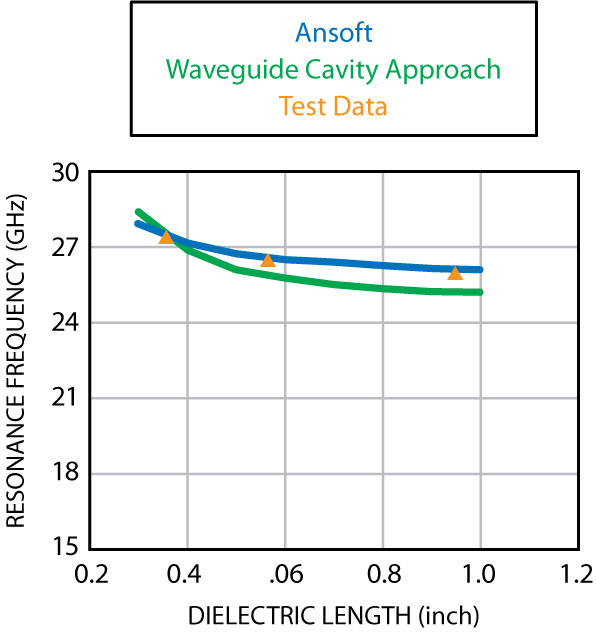
The green line in Figure 3 shows the curve calculated from the waveguide resonator approach. The red triangles show the electrical test data. There are some differences between simulation, calculation and test data but they are not of substantial value. There are other additional factors that can also be considered, such as the slot construction and tolerances, which will also distort the bead effective electrical length, but again, these are not of substantial value. However, the overall field distribution in the area of the dielectric bead is still complicated. There are a few propagating modes at high frequency in the bead area. There is the main TEM wave, there are two TE11 modes and, if the bead is partially filled by dielectric, additional mixed modes. Note that there are not one but two TE11 modes in cross polarization. This is why, in some references, the TE11 (H11) field equation has a component sin x/cos x, (see, for example, Marcuvitz,1 Equation 44). According to Marcuvitz, “…the Hmn-mode (m > 0) may possess either of two polarizations, each characterized by a different voltage and current.” The TE11 mode is not symmetrical in a transverse plane and this is the reason for dual-mode extinction (or in other words, the TE11 mode is degenerate). It can be seen that the exact location of the resonance frequency is interdependent upon many complicated relationships within the connector mechanical and electrical design. It can be seen from the above data that a standard SMA connector cannot be used at extended frequencies without some limitations. When designers needed to enhance the component performance of the SMA connector, extended frequency versions of the SMA connector were designed.7 The resonance frequency in a standard SMA connector is approximately 25 GHz. It can be pushed higher through the incorporation of special design features to create what is known in some companies’ catalogues as a “Super SMA.” The Super SMA family of connectors has been well known for years. These extended frequency connectors are based on modified transverse dimensions of the SMA plug and jack connectors. For example, if both the outer conductor diameter and the effective dielectric constant are reduced, the connector can maintain a 50 Ω impedance while increasing the frequency at which the second mode resonance will occur. This design optimization allows the outer conductor diameter to be 0.154". If the inner conductor diameter stays the same, the cut-off frequency will be increased from 25 to approximately 27.5 GHz. The resonance frequency will increase to higher than 27.5 GHz. Thus, the Super SMA connectors are rated up to 27 GHz.
An extended frequency SMA connector product line, called “Premier SMA,” has been designed by Astrolab. There are two main differences when compared to a typical Super SMA design:
The SMA jack connector has a slight difference in dimensions. There is no special plug connector for the Premier SMA. The “Premier SMA” plug is based on the thick wall design8 because it has an increased frequency range. This design also offers a more mechanically reliable connector.

Figure 4 shows a thick wall SMA plug on the left.
The “Premier SMA” plug utilizing the thick wall design has a cut-off frequency of approximately 33 GHz and therefore does not need any additional features for extended frequency. The resonance frequency is even higher than 33 GHz.
Figure 5 shows the typical performance of a test cable with thick wall SMA plug connectors. The cable assembly was connected to 2.9 mm test ports and showed a resonance frequency at approximately 39 GHz (a similar assembly with a shorter Teflon bead showed this resonance at 42 GHz).
There is no need to define this connector as a special one because the thick wall plug is the original SMA connector invented by Bendix.
The extended frequency SMA jack connector is much more complicated.
From a mechanical point of view, it is not recommended to reduce the inner conductor diameter to less than 0.050". However, it is possible to reduce both the effective dielectric constant of the Teflon and the outer conductor bore diameter. The Premier SMA design has an effective dielectric constant of 1.73, pushing the ‘cut-off frequency’ up to 28.5 GHz.

The main specification for a Premier SMA connector has the maximum operating frequency as 27.5 GHz because of the safety margin concern. However, the true maximum operating frequency of the Premier SMA connector is found when it is mated with a 2.9 mm connector. In this condition, the maximum operating frequency can reach 36 GHz.
Figure 6 shows the second mode resonance in the connector junction between the thick wall SMA plug and Premier SMA jack.
With all of the advantages of the extended frequency SMA connectors, what design concerns should one be familiar with in their use? The first consideration is price. The thick wall design of the SMA plug connector is equivalent to standard SMA plug connectors in price. However, the extended frequency SMA jack is more difficult to assemble and therefore is generally more expensive.
The second design concern is power handling. The extended frequency connectors have reduced transverse dimensions. Additionally, there are some air gaps in order to reduce the effective dielectric constant. Both factors serve to lower the power handling of the extended frequency connector design. However, in many cases, the cable limits the power handling.

The extended frequency connector truly only makes sense for use in high frequency applications, where the cable will be, by necessity, a smaller coaxial line. Thus, in most cases, the cable dimensions are the limiting factor for power handling. Some cables with a low density dielectric can be more powerful than the connector. In this case, special features can increase the connector power handling, but the connector price will be proportionally higher. The design issues involving extended frequency SMA connectors have been discussed in this article and the design guidelines outlined here can open the door as crossover technologies to optimize other industry standard interfaces. Several companies are already applying this technology to the SSMA connector. Using these design tools, the optimized SSMA connector interface can offer design solutions for applications operating up to 60 GHz with great success and reliability.
Conclusion
Most standard SMA connectors can be rated up to 25 GHz maximum. SMA plugs of a thick wall design can be used at higher frequencies; in some cases the connector theoretical limit can exceed 40 GHz. SMA jacks and plugs other than the thick wall design with extended frequency of operation require special features, which increase the resonance frequency. Connectors without the special features can operate at frequencies higher than 25 GHz; however, in this case the dielectric lines must have their length precisely designed for the specific application. The dielectric line length design under consideration must include the mating connector also. A resonance-screening test needs to be done in conditions as close as possible to the real application. The resonance is not always visible. The resonance magnitude and frequency in real connectors may vary as a function of the dielectric line length. The maximum connector operating frequency should have some reasonable safety margin below the resonance value.
Acknowledgments
The author would like to thank Dr. Vladimir Volman from Lockheed Martin and James Kubota from Southwest Microwave, as well as his colleagues from Astrolab, Stephen Toma, Andrew Weirback and Mike Menegus.
References
- Waveguide Handbook, N. Marcuvitz, Ed., McGraw-Hill, New York, NY, 1951.
- H. Neubauer and F.R. Huber, “Higher Modes in Coaxial RF Lines,” Microwave Journal, Vol. 12, No. 6, June 1969, pp. 57–66.
- IEEE P287 Standard for Precision Coaxial Connectors (DC to 110 GHz).
- IEC 61141 (formerly 1141), Technical Report Upper Frequency Limit of RF Coaxial Connectors.
- J. Kubota, “TNC Connector Meet New Performance Criteria,” Microwaves, February 1981, pp. 77–79.
- J.F. Gilmore, “TE11-mode Resonance in Precision Coaxial Connectors,” General Radio Experimenter, Vol. 40, No. 8, August 1966, pp. 10–13.
- Southwest Microwave and M/A-COM catalogues.
- R. Fuks, “Assessing Distortion at Microwave Interface Junctions,” Microwaves & RF, August 1997, pp. 108–116.
- T. Moreno, Microwave Transmission Design Data, Artech House Inc., Norwood, MA, 1989.
- MIL-STD-348A Military Standard, Radio Frequency Connector Interfaces.
- J. Zorzy, “18 GHz Mode-resonant-free Standard MIL-C-39012 TNC Connectors,” Microwave Journal, Vol. 30, No. 5, May 1987, pp. 365–370.
- R. Fuks, “New Dielectric Bead for Millimeter-wave Coaxial Components,” Microwave Journal, Vol. 44, No. 5, May 2001, pp. 318–329.
- D. Grey, Handbook of Coaxial Microwave Measurements, Copyright 1968 by GenRad Inc.; reprinted by Corning Gilbert.
Teflon is a trademark of DuPont.
Super SMA is a trademark of Southwest Microwave.
HFSS is a trademark of Ansoft.
 Rudy Fuks received his Dipl. Eng degree in radio communication engineering from the Moscow Telecommunications Institute in 1973. He joined the Telecommunications Design Bureau, Moscow, Russia, where he held positions as a lead engineer, chief design engineer and department head. His main interest included the design of passive microwave components, such as coaxial connectors and adaptors, terminations, detectors and antennas. In 1994 he joined Astrolab Inc., Warren, NJ, as an RF design engineer responsible for the design of passive microwave components. He has been director of RF technology since 2002.
