
This article explains the critical role of the conductance parameter when describing the channel frequency response (CFR) of a power line cable. The CFR in Power Line Communication (PLC) is a fundamental function determining bandwidth and, therefore, performance. PLC is important for the future of the Internet of Things and the Smart Grid, and where wireless communication is impossible or too expensive. Modeling CFR requires the determination of power line parameters though measurement. These per unit length (PUL) parameters – resistance R(f), inductance L(f), capacitance C(f) and conductance G(f) are frequency dependent. The conductance parameter G(f) is usually neglected in the conventional CFR computation. This work shows that G(f) is critical in determining the CFR on a power line cable. Two types of power line cables are measured – 0.8 mm2 twisted pair and 1.5 mm2 flat twin and earth. An analytical CFR is determined using transmission line theory. Using the PUL parameters in the CFR equation, the analytical CFR is compared to the measured CFR. These conform within experimental limits showing that the analytical CFR is a valid representation. Setting G(f) = 0 in the analytical CFR shows how the bandwidth deviates if the conductance is not included in the CFR calculation.
It is envisaged that in the future, electrical power networks will be part of the “Smart Grid.” This implies that loads and networks will have intelligence and schedule power usage to avoid excessive peak demands.1 In such a smart grid, each load point becomes a network node.2 Not only does each node consume power, but it can communicate on a network of nodes.3 This network of nodes can either communicate via RF (wireless) or through the power line that connects the loads. The last option is known as PLC.4, 5
PLC has the advantage of simultaneously supplying power as well as an electronic communication channel on a cable.4 It is especially suited to use cases of nodes near to each other and where the cost of a wireless link is not feasible.3 PLC performance becomes important if the projection of billions of nodes for future networks becomes a reality.3
Figure 1 conceptually shows two personal computers each connected via a PLC modem through a power line. This power line is noisy and lossy.4 It also has a frequency characteristic known as CFR.
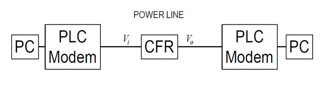
Figure 1 PLC and CFR.
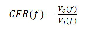
CFR is the output obtained from the power line cable over the input as a function of frequency.6 With reference to Figure 1, this means:
In this work, low voltage indoor power line cables are investigated and their suitability for communications in terms of the CFR is determined. The performance of a PLC channel is directly related to its CFR. Consider Shannon’s theorem,7 which accepts that every transmission channel has a specific capacity determined by its bandwidth, or in this case, its CFR.8 The Shannon-Hartley relationship is given as:7
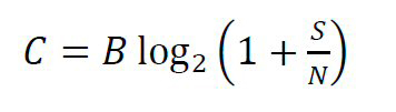
The upper channel capacity limit (C in bits per second (bps)) is directly proportional to the bandwidth B of the channel (measured in Hz), which is the bandwidth of the CFR. The channel capacity is limited by the bandwidth and the level of the signal (S) and noise (N). The signal-to-noise ratio determines the quantity of information that can be transmitted, depending on the signal power and noise characteristics of the channel.
It will be shown that the CFR of a cable is a function of the cable line parameters,6 namely resistance (R), inductance (L), capacitance (C), conductance (G) and cable length (L). It will be argued that all the parameters play a role in the CFR and that G plays a critical role.9
The reason this work focuses on conductance is that it is often neglected in transmission line literature and assumed to have no influence on the transfer characteristics (in this case, CFR) of a cable. Traditional texts neglect the conductance parameter of power line cables and consider the capacitance parameter as constant.10, 11
This implies that a conventional computation of CFR as indicated in traditional texts includes only resistance, inductance and capacitance parameters. Subsequently, inaccurate computation of the CFR of a power line cable occurs due to imperfect insulation, which increases the conductance parameter. This work suggests that it is possible to accurately compute the CFR. It sets up a function for the CFR using telegraphers equations and it investigates conductance parameters and subsequent associated losses, including dielectric losses, dielectric constant, loss tangent and resonance in the computation of an approximate CFR.
In the next section, it is shown how R, L, C and G (the PUL parameters) can be obtained using open and short circuit measurements.6, 9, 11-15 This is followed by a determination of the frequency dependence of R, L, C and G PUL parameters. Then the CFR is calculated using classical transmission line theory.
Measurements and calculations for the CFR of a cable are compared. The direct CFR measurements show good correlation with the calculated CFR. Using the calculated CFR and omitting G shows how the CFR deviates from its correct (measured) value and underscores the criticality of the G parameter.
CIRCUIT REPRESENTATION AND LINE PARAMETERS
The length (ℒ) of a cable determines whether the cable is modeled as a lumped circuit or a transmission line.16 When the frequency of the signal on a cable has a wavelength comparable to the total cable length, the cable is said to be electrically long. When the wavelength of the signal on the cable is much larger than the length of the cable, the cable is said to be electrically short. An electrically short cable can be modeled using lumped circuits, while an electrically long cable acts as a transmission line.
Figure 2 shows a lumped circuit model of an electrically short cable. The equivalent circuit contains a series resistance R and series inductance L. It also contains a parallel capacitance C and parallel conductance G. R is due to the conductivity along the length of the line, while magnetic field coupling along the length of the line causes L.17 Because of the relative proximity of two conductors of a power line, C exists between them.9 Between the two conductors is a dielectric. Leakage across this dielectric causes G.8
Figure 3 shows an infinitesimal representation of a uniform transmission line. The components R1, L1, R2, L2, C and G do not represent single components but rather values PUL. These are the PUL parameters. In the remainder of this article, R, L, C, and G are resistance, inductance, capacitance and conductance PUL.
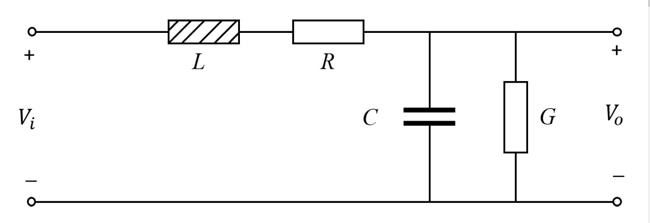
Figure 2 Lumped RLCG equivalent circuit of a cable that is electrically short.
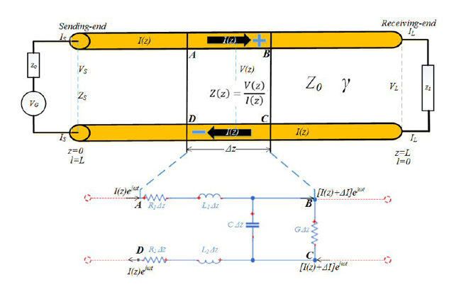
Figure 3 Infinitesimal representation of a uniform transmission line.
The difference between a transmission line and a lumped circuit is that with a transmission line, voltage and current are not only a function of time but also of distance or position on the line. In this work, the PUL parameters are measured and computed using frequencies and electrically short cable lengths. It shows that the computation of CFR cannot be done without considering the frequency dependence of the transmission line PUL parameters R(ff), L(f), G(f) and C(f).
A power line cable line can be characterized by a two-test approach.11, 13 The first is an open-circuited test to determine G(f) and C(f) and the second is a short-circuited test to determine R(f) and L(f). This is shown diagrammatically in Figure 4.
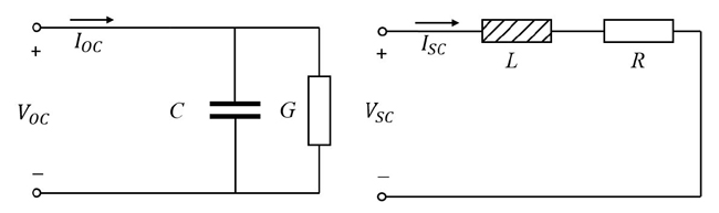
Figure 4 Open and short circuit measurements for characterizing a power cable.
Short-Circuited Test
Figure 4 shows how a short circuit test shorts the capacitance and conductance of a cable. The short circuit voltage (Vsc(f)) and current (Isc(f)) are measured across the frequency range. The PUL resistance is measured as:
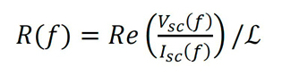
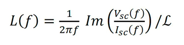
Where ℒ is the length of the cable. The PUL inductance is measured across the frequency range as:
Open-Circuited Test
Figure 4 shows how an open-circuit test can be used to determine the capacitance and conductance of a cable. The assumption is that because of the low load and low current drawn by the shunt C and G elements, the voltage drop across R and L is negligible. The open circuit voltage (Voc(f)) and current (Ioc(f)) are measured across the frequency range. The PUL conductance is measured as:
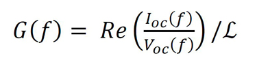
Where ℒ is the length of the cable.
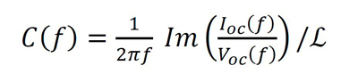
The PUL capacitance is measured across the frequency range as:
PUL PARAMETER ESTIMATION
A transmission line can be characterized by a two-test approach. The first is an open-circuited test and the second is a short-circuited test. The first test (open circuit) is used to determine the PUL conductance and capacitance of the line. The second (short circuit) determines PUL resistance and inductance. A precision impedance analyzer is used to measure and analyze the PUL parameters from 40 Hz to 110 MHz. Two types of power cables are measured, a 0.8 mm2 twisted pair and a 1.5 mm2 flat twin and earth.
Open-Circuited Line
Figure 5 shows the measured admittance in siemens per meter for open-circuited 10 m cables. It contains both the magnitude and relative phase. Below 10 kHz, the measurements seem to be very noisy. This is because there is little current and the process of current measurement is prone to noise. Up to around 1 MHz, the admittance seems to follow nearly a straight line. For this frequency range, the cable is electrically short. Above 1 MHz, the cable becomes electrically long, and transmission line effects are seen.
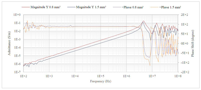
Figure 5 Open-circuit admittance measurements in siemens per meter for 10 m cables.
Figure 6 shows the PUL conductance in siemens per meter for different 1 m cables. It is calculated from Equation (5). It is clearly seen that the conductance is a function of frequency. The conductance changes by several orders of magnitude over the measured frequency range. At low frequencies, the dielectric insulation in the cable is very effective, and the conductance is low. At higher frequencies, different mechanisms cause the dielectric strength to increase and conductance increases. It is seen that conductance follows straight lines on the logarithmic scale of the graph. These functions are noted and used as G = G(f). A numerical expression for conductance is used in the remainder of this work.
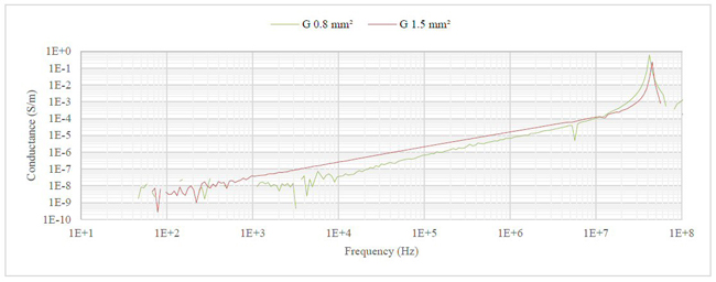
Figure 6 Open circuit conductance in siemens per meter for 1 m cables.
Figure 5 shows results for 10 m cables and Figure 6 shows results for 1 m cables. In both, transmission line effects alter the straight line where the cable is electrically short and can be modeled as a lumped circuit. The expression (G(f)) used later to calculate CFR ignores transmission line effects and follows the straight line for conductance into the electrically long (transmission line) area of the graph.
Figure 7 shows the open circuit PUL capacitance in farads per meter for 1 m cables. It is calculated from Equation (6). Up to around 10 MHz, the capacitance is fairly constant. At higher frequencies, the cable is electrically long and transmission line effects influence the reading. In modeling the capacitance (C = C(f)), transmission line effects are ignored and the capacitance is defined as a straight line extending the sub 10 MHz values.
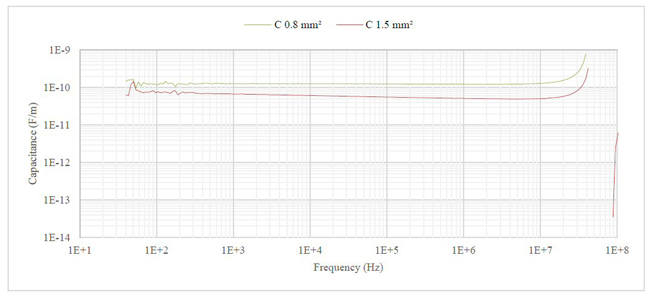
Figure 7 Open circuit capacitance in farads per meter for 1 m cables.
Short-Circuited Line
Figure 8 shows the results of the PUL impedance in Ω per meter for short-circuited 10 m cables. It contains both the magnitude and relative phase. Up to around 1 MHz, the impedance seems to follow a typical function for a resistor with skin effect.18-20 For this frequency range, the cable is electrically short. Above 1 MHz, the cable becomes electrically long, and transmission line effects are seen.
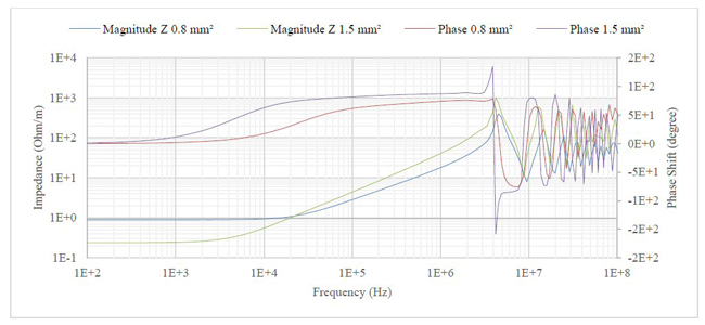
Figure 8 Short circuit impedance in Ω per meter for 10 m cables.
Figure 9 shows the short circuit PUL resistance in Ω per meter for 1 m cables. It is calculated from Equation (3). Up to around 10 MHz, the resistance follows a typical function for a resistor with a skin effect. At higher frequencies, the cable is electrically long and transmission line effects influence the reading. In modeling the resistance (R = R(f)), the transmission line effects are ignored.
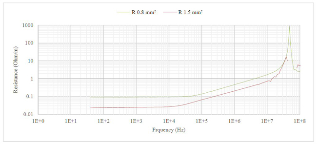
Figure 9 Resistance in Ω per meter for 1 m cables.
Figure 10 shows the short circuit PUL inductance in henries per meter for 1 m cables. It is calculated from Equation (4). Up to around 10 MHz, the inductance follows a fairly straight line. At higher frequencies, the cable is electrically long and transmission line effects influence the reading. In modeling the inductance (L = L(f)), the transmission line effects are ignored.