
SYSTEM DESIGN AND SIGNAL PROCESSING
Range Processing
Signal processing is at the heart of an FMCW radar. In an FMCW radar, the frequency of the transmitted signal is linearly modulated with time; such signals are called “chirps.” An FMCW radar measures the distance of an object using the time delay between the transmitted chirp and the received chirp. This time delay manifests in the base band as a sinusoidal frequency. Thus, the frequency of the received base band signal is proportional to the time delay and hence proportional to the range of the object. The maximum distance “seen” by the radar is a function of the ADC sampling rate and chirp sweep bandwidth. Steradian uses analog transmitter beamforming techniques in conjunction with a careful selection of the ADC sampling rate and chirp sweep bandwidth to further enhance the maximum range. The present generation platform can detect objects well beyond 300 m (see Figure 3) with the goal of detecting objects up to 400 m and beyond. The sweep bandwidth for these chirp signals is 76 to 81 GHz. The chirp sweep bandwidth dictates the achievable range resolution.
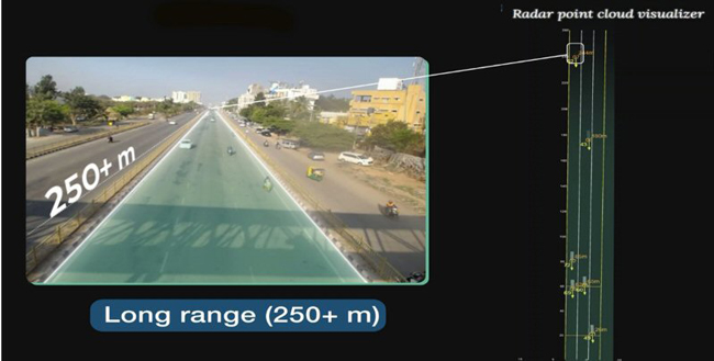
Figure 3 Imaging radar long range detection.
Velocity Processing
The signal model for an FMCW radar consists of several transmitters each transmitting a certain number of chirps. The biggest advantage of a radar sensor with respect to other sensors, like camera and lidar, is that it can measure the radial velocity of an object. The velocity information is embedded in the sequence of chirps received (see Figure 4). The ‘inter-chirp’ time, i.e., the time delay between successive chirp transmissions dictates the maximum unambiguous velocity that the radar can measure, while the total duration of the chirps dictates the maximum achievable velocity resolution. Using sophisticated signal processing and data science techniques, both the maximum achievable unambiguous velocity as well as velocity resolution can be further enhanced. Steradian’s radar solution can deliver a velocity resolution of 1 km/h and a maximum unambiguous velocity of 320 km/h, challenging existing benchmarks and specifications.
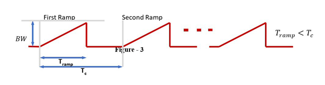
Figure 4 Typical FMCW radar ramp sequence.
Direction of Arrival (DoA) Estimation
A typical radar RFIC consists of three to four transmitters and receivers. Together they form a MIMO virtual array. A MIMO virtual array is the number of transmit (Tx) channels times the number of receive (Rx) channels. The physical spacing/separation between the MIMO channels dictates the maximum measurable unambiguous angle of the detected object, and the total aperture size of the MIMO array dictates the best achievable angular resolution.
Angular resolution is the ability to resolve two objects at the same range with the same radial velocity. Sometimes there is a need to resolve objects separated by less than 1 degree. In such cases, a single RFIC MIMO array will not suffice. It is this requirement that drives a cascaded solution where three to four radar RFICs are cascaded, increasing the total number of MIMO virtual channels, hence improving the angular resolution.
As in the case of velocity, angular resolution can be enhanced using high-resolution spectral estimation techniques; however, these methods are computationally intense and require spatially filled MIMO grid arrays. Filled MIMO arrays have their challenges in terms of routing lengths and bends, for example. Sparse spatial MIMO arrays are a solution. Sparse sensing techniques such as basis pursuit and matching pursuit can be used, but these algorithms have associated challenges as well, in terms of computational complexity and convergence.
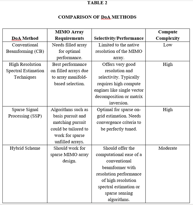
Steradian employs a mix of spatially sparse MIMO arrays (which offer routing advantages) with high-resolution spectral estimation techniques (which offer best resolution performance). These innovations deliver a sub-1 degree angular resolution. The solution’s high elevation resolution allows the detection of bridges, vehicles under bridges and manholes, which is not possible with conventional radar. Table 2 compares different DoA methods, listing their pros and cons.
The size of MIMO arrays is typically in the range of 192 to 256 virtual array elements. More important than the number of virtual MIMO channels, however, is the actual placement of the Tx/Rx elements. Figures 5 and 6 show how MIMO virtual channels can be used to obtain either a filled array of lower aperture (lower angular resolution) or a sparse array having larger aperture (higher angular resolution) for the same hardware channel count. By using a hybrid of these two kinds of arrays, the best of both worlds can be achieved.
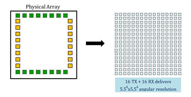
Figure 5 A sixteen Tx and sixteen Rx array can be arranged to produce a filled (dense) array with lower angular resolution.
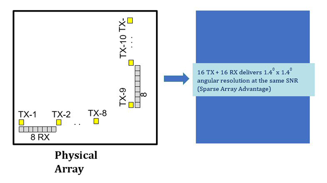
Figure 6 A 16 Tx and 16 Rx array can be combined differently to get two 64-element uniform linear arrays: a horizontal 64-element array can be used for azimuth angle estimation and a vertical, or a vertical or tilted (known tilt) 64-element array can be used for elevation angle estimation.
Tracking and Classification
Once an object’s range, velocity and angle are estimated, its position coordinates (X, Y, Z) (also referred to as its point cloud) can be known. With improvements in angular and range resolution leading to a much denser point cloud, Steradian has shown that a radar sensor can function as a truly 4D imaging solution. This point cloud output together with other attributes from the radar, such as radial velocity, provides a cornucopia of rich information about the surroundings, which can be harnessed for a variety of applications.
Object tracking is one such application, where the point cloud and the radial velocity can be used to predict the heading and velocity of vehicles such as cars, bikes and trucks. This is particularly useful when there are no radar reflections from a vehicle due to occlusion by other objects/vehicles for a short period of time.
The intensity of the signal received at the radar due to reflections from surrounding objects carries information about the type of object. For example, the signal received from a large metallic object like a truck is very strong as compared to a signal reflection from a small bike. Thus, different objects reflect different amounts of incident signal power. This attribute of an object to reflect a fraction of the incident power is characterized by a parameter called radar cross section (RCS).
The RCS of a 12-wheeler truck is much larger than the RCS of a two-wheeler bike. Hence, this parameter serves as one of the tools to distinguish a truck from a bike or a car from a human. Steradian harnesses all the received radar signal features to glean object attributes and classify them as pedestrians, VRUs, bikes, cars, trucks and other objects. A classification accuracy of about 95 percent has been demonstrated for different categories of vehicles.
Thus, the fundamental radar output with the help of complex signal processing and machine learning techniques can be used for applications such as high-definition 4D imaging, vehicle tracking, lane change estimation, collision avoidance and classification. This information rich output is characteristic of a true imaging radar (see Figures 7 and 8).
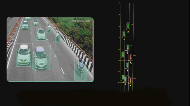
Figure 7 Illustration of the imaging radar’s tracking performance showing the ability to track and identify hundreds of vehicles simultaneously with high accuracy.
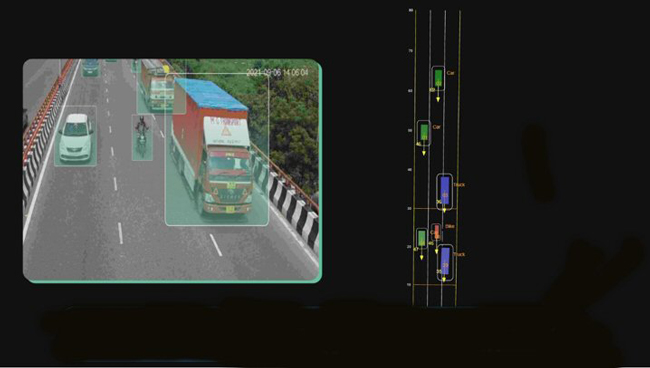
Figure 8 Illustration of the imaging radar’s classification performance showing three types of vehicle classification at 95 percent accuracy (software upgradable to higher classes).
CONCLUSIONS
The performance of an imaging radar solution is dictated by careful design of system parameters like ADC sampling rate, chirp sweep bandwidth, chirp slope, inter-chirp time, number of chirps, number of receiver elements and receiver element spacing, to name a few. Steradian has shown that with an innovative and efficient design of these system parameters, the imaging radar solution can be used for a myriad of applications such as intelligent transportation, automotive, vital sign (heart rate, breathing rate) monitoring, security/surveillance and level sensing.
The ability to conduct lane change estimation, ego-velocity estimation, vehicle classification, estimation of vehicular density and so on are examples of the developments that have enabled newer applications. The imaging radar described here delivers a real-time solution of 20 FPS for its high-density point cloud output. The software stack is processor agnostic and can run on off-the-shelf GPU or DSP platforms. It provides a differentiated radar solution both in terms of its hardware and software stack.
This video shows the imaging radar’s dynamic performance.