
The concept of self-phase-locking12 is also shown in Figure 3, i.e., the loop with the GPLL path. In the self-phase-lock loop (SPLL) process, a portion of the oscillator output is delayed, and the phase of the delayed signal is compared to the phase of the current signal. The comparison signal is amplified by an operational amplifier and fed back to the VCO tuning port (e.g., the voltage control of the PM portion of the MML). The feedback frequency control is initially a low frequency signal of up to 30 MHz and eventually settles at a DC signal when no frequency error is detected between the delayed and non-delayed signals.
With the principal of superposition applied, the overall noise of the SPLL system is12

Combining the SIL and SPLL leads to the SILPLL with a similar simplified expression,16 conceptually shown in Figure 3. In this topology, the SIL and SPLL operate at the same time with separate external delay circuits. The derived expression using superposition is

where
Equation 3 signifies that the SIL, SPLL and their combination significantly reduce the phase noise without any external reference.
The setup to test the SIL is shown in Figure 4, where the instantaneous laser output is amplified using a constant gain, erbium-doped fiber amplifier (EDFA). The output is delayed by 25 μs using a 5 km fiber and fed back to the laser through an optical circulator. A tunable optical attenuator placed before the optical circulator port enables the dynamic performance to be evaluated by adjusting the optical injection power level. A polarization controller after the optical delay line provides a high efficiency optical injection signal to the optical waveguide.
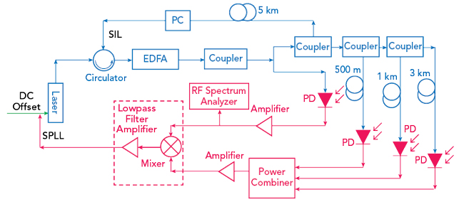
Figure 4 Inter-modal oscillation stabilization using SIL and triple self-phase lock loop (TSPLL).
The performance parameters of phase-locking range and time to pull-in to phase-locking state17 for the SPLL is enhanced when SIL is incorporated to SPLL. The delayed and non-delayed signals are simultaneously compared in a phase detector that is realized using a mixer and lowpass filter amplifier (see Figure 4). Any instantaneous low frequency phase error pulls the frequency deviation back to the original RF oscillation phase-locking using the PM section of the MML. The PLL loop bandwidth of 50 MHz was selected to completely cover 30 MHz of frequency drift. Different offset bias conditions of the PM section were compared using optimized self-injection locking 5 km and triple, self-phase-locking 0.5, 1 and 3 km delay lines to test the phase noise (see Figure 5). Triple non-harmonically related delay loops16 suppress the peaks of the side modes from -30 to -90 dBc. In the best scenario, the timing jitter was 0.448 ps, 600x better than the free-running jitter. The accuracy of self-forced oscillation modeling results are validated and experimentally reported for phase noise of both DRO11-14 and optoelectronic oscillators.4
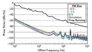
Figure 5 Simulated vs. measured phase noise of self-forced SILPLL-stabilized inter-modal MML oscillator vs. bias. SIL: 5 km, STPLL: 500 m/1 km/ 3 km. Carrier frequency = 11.54 GHz, 3.59 dBm output. Free running oscillator shown for comparison.
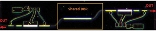
Figure 6 Shared DBR-based multimode semiconductor laser with symmetric multi-section multimode lasers on the left and right of a shared DBR. Chip dimensions = 4.6 mm x 1.2 mm.
FREQUENCY SYNTHESIS USING SML
To achieve broadband frequency synthesis, two MML pairs (see Figure 1) were configured to produce counter-propagating laser light feedback to form an RF synthesizer (see Figure 6). This SML process7 combined with frequency detuning the multimode laser sections easily provides tunable RF beat notes. Figure 7 shows a block diagram of this novel SML method, which does not rely on standard active mode-locking where an external frequency reference is required. The symmetric outputs of multi-section laser pairs interact as two counter-propagating feedback waves. The larger the number of modes locked to one another, the lower the close-in phase noise, i.e., the better the RF frequency stability.7,8
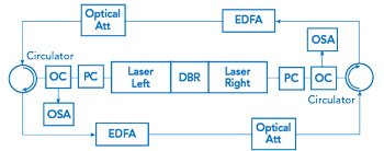
Figure 7 SML method with two counter-propagating feedback waves of symmetric laser pairs. The current realization uses modular components off the InP chip.
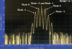
Figure 8 Five modes shown on an optical spectral analyzer.
The SML technique forces one laser output to be coherent with the other by locking the overlapped modes of the counter-propagating lasers, as bias currents of the SOA and voltages of the PM and EAM are tuned through the shared DBR and added external feedback. As shown in Figure 7, the amplified outputs from the left and right lasers are coupled back to the opposite lasers through optical circulators. The optimum level of light coupling is quantified by feedback power levels (e.g., an EDFA with optical attenuator). The measured fundamental mode of the two lasers with their intermodal gap is approximately 2.1 Ao (i.e., 26.4 GHz) for each laser. The spectra of the correlated modes is shown in Figure 8. Mode +1 of the left laser overlaps with mode -1 of the right laser, which provides exactly five modes that are correlated. The best interaction of five locked modes of intermodal oscillations at 26.4 GHz achieves a measured phase noise of -92 dBc/Hz at 10 kHz offset, which is a 55 dB improvement compared to the free-running case. The estimated timing jitter is 72 fs, 1000x lower than the estimated 70 ps for the free-running case over a bandwidth of 1 kHz to 1 MHz.
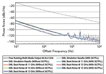
Figure 9 Phase noise for beat-notes at 11, 12 and 13 GHz with five self-mode locked modes,7 with and without the SILTPLL.8 Measured and modeled results reported by Sun also shown.18
To achieve RF synthesis, continuous wavelength tuning of the laser section is used after achieving mode-locked status, by tuning the SOA and PM to produce different beat notes. During this process, the laser modes remain locked. By tuning each laser section, the intermodal oscillation frequencies are tuned to 11, 12 and 13 GHz with RF power levels of 4.79, 4.80 and 4.70 dBm, respectively. The related phase noise and a comparison to analytical modeling are shown in Figure 9.