
Many electrical components have wide performance specifications to allow for high yield in production testing. Such an approach, however, comes at a cost. The problem is the outliers, the out-of-family components which pass the electrical specifications but are noticeably different from the rest of the population. These outliers, which represent anywhere from 0 to 4 percent or so of the passing units (depending on the specific definition of an outlier), can often be identified when the data is analyzed in its entirety, post measurement. However, at this point, it may be impossible to separate the outliers from the “pass” population, especially if the units have been placed in storage, such as on tape and reel. Therefore, a preferred approach is to identify and remove outliers in real-time during the production test.
Outlier detection of integrated circuits has been examined in the past as detailed by Stratigopoulos.1 Here, the author presents a thorough discussion of outlier detection via machine learning, though the specifics of implementing a detection algorithm are not discussed. Others, such as Yilmaz,2 have used outlier analysis to reduce the defective parts per million and the production test time. Jauhri3 discussed the identification of outliers at the wafer level and used this information to unearth problems in the manufacturing process. Bossers4 considered a univariant, real-time approach to detect outliers in production on a rolling basis, but under the assumption the units always followed a normal distribution. Finally, O’Neill5 considered outlier detection using just one measured parameter, though this technique was intended for post-processing and not real-time.
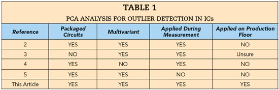
Table 1 has a summary of this previous work. As shown in the table, the previous work does not adequately address outlier detection on the production floor. Therefore, this article presents a real-time method for outlier detection using principal component analysis (PCA), beginning by describing the theory behind PCA. Next, we deploy PCA in a post-processing role to examine its ability to detect outliers, then describe a real-time implementation of a PCA algorithm on the production floor, showing the results. Finally, we offer conclusions and plans for future work.
PCA AND OUTLIER DETECTION
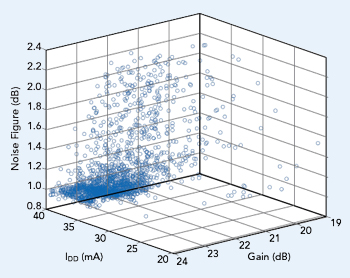
Figure 1 Gain vs. noise figure vs. IDD for 2,139 CMD132P3 LNAs.
PCA is a statistical method used to discover and quantify relationships between variables in a data set.6-7 Consider a set of measurements, S, organized into an m x n matrix, where each of the m rows represents the measurement of one unit over n parameters.
For example, the CMD132P3, a commercially available low noise amplifier (LNA) from Custom MMIC, has n = 3 measured parameters: gain, noise figure and supply current (IDD). From experience, we know there is some correlation between these parameters: if the gain of the CMD132P3 is low, the noise figure may be higher than average; if the current is high, the gain may be high as well. But this correlation is not easily identified. Figure 1 is a scatter plot of gain versus noise figure versus current for one lot of CMD132P3 LNAs (m = 2189 units). Each circle in the figure represents a unit that passed the electrical specifications. Note the data is not clustered tightly, instead spread over the acceptable range of the three parameters, making it difficult to discern the outliers. With PCA, however, we can quantify the relationship between the measured parameters and more easily discover the outliers.
The first step deploying PCA is to normalize the data in S and generate a new matrix, X. Normalization effectively removes the unit of measure from the data. Without this step, measurements that produce large numbers, such as an IDD of 35 mA, would completely overshadow smaller measured values, such as a noise figure of 1.5 dB, even though each measurement is equally important. Normalization is accomplished through a straightforward calculation:
Here, (i,j) is the row and column identifier of the elements in X and S, Sj is the mean of column j, and σj is the standard deviation of column j, where j = 1, 2, ..., n, and i = 1, 2, ..., m. The result of this normalization is each column of X now has zero mean and a standard deviation of 1. Once X has been generated, the covariance matrix, X*, is formed:
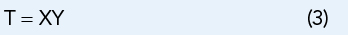
We then find the eigenvalues and eigenvectors of X* and sort the column eigenvectors by the highest to lowest eigenvalue, creating a new matrix, Y. The columns of this sorted matrix, Y, are referred to as the principal component axes. Formally, matrix Y is an orthonormal set of basis functions (i.e., principal components) onto which we can project the normalized measured data. Matrix Y is also called the PCA coefficient matrix. Once we have generated the coefficient matrix, Y, we determine the PCA score matrix, T, for the data set through a simple matrix multiplication:
Matrix T is an m x n matrix, the same size as the initial data set, S, and each row represents the projection of the normalized measured data onto the n orthogonal principal components. Outliers will generate high scores in their respective row of the matrix T, where normal or typical measurements will generate low scores. We can then set a maximum PCA score to remove the outliers from the population.

REAL-TIME PCA ALGORITHM
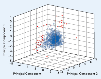
Figure 2 T-matrix scores for the LNAs from Fig. 1, showing the outliers in red.
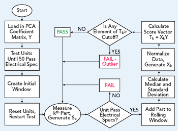
Figure 3 PCA algorithm for real-time outlier removal at production test.
Figure 2 plots the elements of T from the CMD132P3 data set used to create Figure 1. The majority of the measured data is clumped around the (0,0,0) coordinate, and a number of outliers (shown in red) can clearly be seen on the fringes of the graph. For this example, the outliers were defined as having a PCA score greater than 7. Analyzing several different LNA data sets using this same approach, in all cases the T-matrix scores identified outliers in a similar manner. For reference, Table 2 provides a summary of the variable definitions and their matrix sizes.