
Methods of radio signal filtering, summing and separation in the frequency domain are widely used during signal generation and processing. The implementation of filters with high quality factors (Q) up to frequencies in the mmWave range is challenging. Frequency filtering can be achieved through analog means (in hardware) or digitally (in software). This discussion considers only analog frequency filters in the RF, microwave and mmWave frequency ranges.
A frequency filter is a linear electrical circuit with lumped or distributed parameters. A frequency filter is generally characterized by the complex transfer coefficient Ẇ(f), which can be described by amplitude-frequency | Ẇ(f )| and phase-frequency φ(f ) = arg[Ẇ(f)] characteristics (AFC and PFC, respectively). The function Ẇ(f ) describes the pulse response h(t) at the filter’s output after applying a short pulse (impulse) to its input. The slope of the filter PFC defines the group delay (tgroup) of the response, which depends upon frequency
tgroup = - (1/2p)(df/df) (1)
The ideal nondistorted filter has one or several bandwidths, for which the ideal transfer coefficient modulus |S21(f)| = 1 and one or several suppressed bands (rejection), for which the ideal transfer coefficient is equal to zero. Ideally, a signal whose spectrum width is narrower than the filter bandwidth is reproduced without loss or distortion at the output, but with a time delay.
Physically realizable frequency filters have loss at their bandwidth boundaries (cutoff frequencies) and AFC ripple within their bandwidths; this causes frequency distortion in the output signal due to PFC nonlinearities. They also have finite gain slopes at their bandwidth boundaries, and accordingly, finite group delays.
Filters are classified according to the location of passbands and attenuation bands, the character of amplitude-frequency and phase-frequency characteristics, selectivity, topology of construction and manufacturing technology. The main classes are lowpass filters (LPF), highpass filters (HPF), bandpass filters (BPF) and band-reject filters (BRF).
The band-reject or band-stop filter has the combined characteristics of a LPF and a HPF; a notch filter is a BRF with a narrow stopband (i.e. a high Q). More complicated/combined filtering products include multiplexers (diplexers and triplexers), duplexers, dispersive filters, preselectors, tunable and switchable filters and filter banks, filter-amplifiers, filter-couplers, and duplexer-filter/low-noise amplifier assemblies.
The complex filter transfer coefficient Ḣ can be represented by the ratio of polynomials of the Laplace operator p = σ + j2πf
Ḣ = (a0 + a1p + … + aMpM)/(bo + b1p + … + bNpN); N>M (2)
Here a0, a1,…, aM, b0, b1,…, bN are constant coefficients, M and N are integers indicating the number of zeros and poles in Equation 2. Their mutual locations on the complex plane and quantitative values determine the main parameters of the AFC and the PFC (e.g. shape-factor, in-band ripples and pulse response). N is the filter order.
FILTER RESPONSE CHARACTERISTICS
The following amplitude characteristic responses are typical: Chebyshev-1 or Symmetrical Equiripple Lumped Filter (SELF). The Chebyshev filter is arguably the most popular filter response type. It provides the greatest stopband attenuation but also the greatest overshoot. It has the worst group delay flatness.
Bessel (maximally flat group delay). This filter has the best in-band group delay flatness, with no overshoot, but the lowest stopband attenuation for a given order, and percentage bandwidth. It is ideal for receiver applications such as image-rejection filters.
Butterworth (maximally flat amplitude-frequency characteristic). This filter has the best in-band amplitude flatness, but has lower stopband attenuation than a Chebyshev filter; it is better than Chebyshev for group delay flatness and overshoot and is usually used as a compromise. It is common to use a Butterworth lowpass filter, which gives a continuous and monotonic response without discontinuity and without ripples in the frequency domain. The equation for a Butterworth lowpass filter is given by:
| Ẇ(f )| = 1/sqrt (1 + (f/fcutoff)2N) (3)
where fcutoff is the cutoff frequency and N is the filter order (the order is determined by the number of capacitors and inductors in the circuit). The Butterworth highpass filter is similar; the only difference is that the fraction in the denominator is inverted:
| Ẇ(f )| = 1/sqrt (1 + (fcutoff/f)2N) (4)
All of the above filters are realizable in parallel-coupled, direct-coupled and interdigital filter topologies.
Elliptic or Cayer is a filter whose transfer function is derived through the use of Jacobean elliptic functions. The amplitude is equal ripple in both the passband and stopband. This type of filter offers the most selectivity per pole but has the worst delay and phase linear performance. These filters can sometimes be designed wider than Butterworth or Chebychev filters thereby offering reduced insertion loss.
Gaussian. This filter provides a Gaussian response in both frequency and time domains and creates minimal group delay time. Its transfer characteristic g(t) has no overshoot:
g(t) = (BW-3dBT)(2p/sqrt(ln 2))exp[-(2p2(BW-3dBT)/T2ln2)t2] (5)
where BW-3dB is the bandwidth at half-power and T is the time characteristic.
Linear phase. This filter has a maximally linear PFC. For example, with N = 8 at a center frequency of 100 MHz and with a relative bandwidth of 5 percent in the frequency band 75 to 125 MHz one may obtain over 540 degrees of phase, a deviation from linear of not more than 3 degrees (see Figure 1).
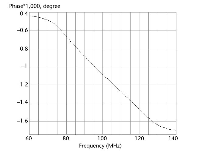
Fig. 1 Phase-frequency characteristic of a highly linear BPF.