
DESIGNING FOR POWER AMPLIFIER EFFICIENCY: STATISTICAL DESCRIPTION OF SIGNALS
Multichannel amplifiers have become ubiquitous in modern communications, including cellular, satellite and other wireless systems. While power efficiency is well understood for CW signals, the amplitude of multicarrier signals varies in time. Today's component designers must be able to simulate and analyze this kind of varying-envelope signal in order to develop successful devices cost effectively - a task entirely within the realm of today's advanced simulation tools.
This article explores the properties of baseband multicarrier signals. The concept of power-added efficiency (PAE) for these signals is defined and the statistical approach to signal description is introduced. This approach estimates signal levels and enables the application of classical computation concepts to signals with randomly varying power. Ultimately, this yields closed-form formulas that can be used to describe the PAE of class A and B amplifiers.
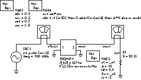
Fig. 1 Class B amplifier model.
To facilitate the discussion, amplifier models are kept simple to allow concentration on signal descriptions and input-output characterization results. Thus, the primary goal will be the analysis of power levels in the baseband signal. Finally, the definition of average PAE will be introduced, as well as an overview of how it enables designers to make intelligent tradeoffs about average efficiency versus linearity.
POWER AMPLIFIER EFFICIENCY FUNDAMENTALS
The simple class B amplifier shown in Figure 1 is modeled by a symbolically defined device (SDD), which enables its input/output relationships to be to specified. Input current (i1) is determined by the admittance Gi.
The output voltage (Vout) is modeled by a voltage source V2 in series with a resistance Ro.
For a class A amplifier:
V2 = if | Vin | < Vsat/A then A x Vin else Vsat x sign(Vin) end if
For a class B amplifier :
V2 = if Vin < 0 then 0 else if Vin < Vsat/ A then A x Vin else Vsat end if
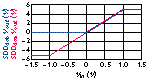
Fig. 2 SDD input/output characteristics for class A and B amplifiers.
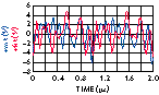
Fig. 3 Two Monte Carlo simulation samples.
The plot shown in Figure 2 illustrates the input/output characteristics the SDD amplifier models from the previous example over a Vin range of -1.5 to +1.5 V. The class A model provides linear gain and clipping at ?Vin? = 1 V. The class B model provides linear gain only for positive signals and clipping at Vin = 1 V.
If a varying power waveform is applied to the class B amplifier, the device only amplifies through half of the cycle. This limits DC power dissipation to half of the cycle and significantly improves power efficiency.
Power efficiency for class A and B amplifiers is well known. The theoretical upper limits of this efficiency can be expressed using the expressions:
Class A: h = Prf/Pdc = 0.5 z
Class B: h = Prf/Pdc = (p /4)vz
Where z represents normalized RF power so that z = 1 corresponds to the maximum power for which the signal is not clipped.
For class A amplifiers, the DC supply is constant and the RF amplitudes cannot exceed the biasing voltage and current. The result is 50 percent efficiency at maximum amplitudes (that is, when z = 1). For class B amplifiers, where the DC power supply depends on the RF output, the results are better than class A amplifiers, reaching a theoretical maximum at p /4, or 78 percent. Real amplifier efficiency is typically 30 percent to 50 percent lower than these limits due to losses in matching circuits and in DC supplies and the nonideal behavior of real devices.
MULTICHANNEL SIGNAL ANALYSIS
Multicarrier signals consist of a number of digitally-modulated carriers with a spacing of several megahertz. Since these types of signals generally use carrier frequencies in the gigahertz range, the baseband "comb" can be thought of as a slowly-varying envelope:
Consequently, the multicarrier signal power is
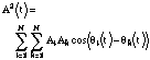
If the signals are phase or frequency modulated, then all amplitudes (Ak) will have the same value. Figure 3 shows a multicarrier signal envelope simulation. Two out of 250 samples from a Monte Carlo simulation are displayed. The envelope contains 10 signals with equal amplitudes and randomly varying phases (with uniform distribution), that are spaced at 1 MHz intervals. Note that the envelope (and consequently the signal power) strongly varies in time and also from sample to sample.
To analyze the probability distribution of the power of multicarrier signals, a signal that contains two carriers only will be used. Figure 4 reveals the simulation results from 250 Monte Carlo samples of the power of a two-carrier signal. The data are presented as a normalized histogram spread over 50 bins. The horizontal axis is envelope power, while the vertical axis shows the number of instances (from the sample of 250) that correspond to each power level.
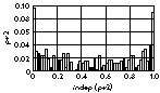
Fig. 4 Simulated two-carrier power distribution.
Fig. 5 PDF for sinusoidal envelopes.

It is apparent from this plot that the signal power remains close to zero and one for much of the time. A similar histogram for a CW signal would have a peak at one, and zeroes elsewhere.
The shape of this plot can also be found geometrically. Indeed, for two carriers with amplitudes equal to one, the power (envelope squared) equals 1 + 1 + 2cosq = 4cos(q/2)2. When transformed through the power of the sinusoidal envelope, z = (cos(x))2 (upper-right plot shown in Figure 5), the uniform distribution of the phase shift x (bottom plot) results in a cup-shaped distribution (upper-left plot).
Consider a 10-carrier signal with equal amplitudes and random (uniformly distributed) phases. The results of Monte Carlo simulation of 250 samples are shown in Figure 6 together with the chi-square distribution. Note the close agreement between the two plots. It is a well established fact that the chi-square is a limit distribution for a large amount of carriers. This fact follows from the central limit theorem, which asserts that many independent random signals added together have a Gaussian distribution. Applying the theorem to in-phase and quadrature carriers two Gaussian processes x and y are obtained. Therefore the signal power of many carriers is the sum of two squared Gaussian processes which means that it has a chi-square distribution (with two degrees of freedom) such that
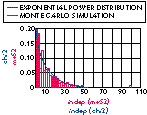
Fig. 6 Theoretical exponential distribution for power vs. a Monte Carlo simulation.
Fig. 7 PDF for Pout.
Consequently, the expected power of the multicarrier signal equals the sum of the carrier's power
Two important conclusions follow: First, the simulation shows that 10 carriers approximate very well the theoretical many-carrier distribution. Also, there is a significant spread in the value for envelope power, as well as non-negligible probability that a given signal will exceed the expected value (up to 10 times higher).
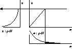
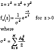
The probability distribution of a multicarrier signal after it passed through an ideal clipping amplifier can now be calculated. If a multicarrier signal is passed through it, in the linear region, the probability distribution remains exponential since the signal is multiplied by a constant. However, all points above saturation are related to the saturation point. In terms of the probability distribution, this lumping of probabilities into one point is represented by Dirac's delta, shown in Figure 7. Clipped signals are indicated by the arrow in the upper left plot. The signals are represented by Dirac's delta distribution, for which the weight is set by the shaded part of the bottom plot.
The analytical expression for this distribution is
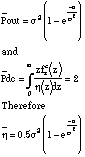
Once the probability distribution is obtained, the average output power can be found as

and the probability of the clipped signal is e-a/s2
It is convenient to use h(z) to find mean Pdc:

Consequently, the average efficiency can be calculated using: h = P_out/P_dc.
Thus, for a class A amplifier

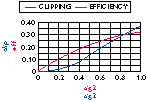
Fig. 8 Average efficiency vs. linearity.
with clipping probability e-a/s2
It is already known how much clipping is obtained for a given signal level and the amplifier's saturation level. Thus, a tool now exists that enables us to precisely measure the amplifier's efficiency and linearity, and consequently make tradeoffs of one versus the other.
The plot shown in Figure 8 compares the loss of linearity (probability of clipping) and the average efficiency. It is assumed that amplifier saturation is fixed (normalized to one), and that sigma-square is being changed. This condition corresponds to the situation when the amplifier is fixed and the signal level is controlled.
What is found is that as the mean power reaches 20 percent of saturation, the percentage of the clipped signal is approximately one percent, while the average efficiency reaches 10 percent. Of course, the actual signal level will vary depending on the application.
CONCLUSION
The tools described enable amplifiers to be designed in the presence of many signals with random phases. In particular, amplifier linearity versus power efficiency can easily be balanced. While the examples shown are very simple, the methods are applicable to many kinds of amplifiers with a range of saturation characteristics. The analysis methods presented can easily be generalized for class B amplifiers, where mean Pdc is expressed by erf(a), as well as for class AB and C amplifiers with the use of slightly more complex expressions. Finally, as shown, distributions can be calculated numerically via Monte Carlo analysis.
ACKNOWLEDGMENT
The author wishes to thank Wolfgang Bosch at Filtronics plc., for permission to use his notes.