Three-Sampler Network Analyzer Calibrations

TECHNICAL FEATURE

THREE-SAMPLER NETWORK ANALYZER CALIBRATIONS

DRAGO KOSTEVC AND JOZE MLAKAR

University of Ljubljana

Ljubljana, Slovenia

Calibration is the most important aspect of measurement with a network analyzer. The standard method for network analyzer calibration is short-open-load-through (SOLT) calibration.1 For calibration of four-sampler analyzers, the use of self-calibrating procedures is also possible in addition to the SOLT calibration. With self-calibration, fewer standards need to be measured during calibration, or a line is used instead of a matched load as a non-reflecting standard, which is particularly useful for calibrating analyzers with non-standard connectors. However, the use of self-calibrating procedures is restricted to four-sampler analyzers.2

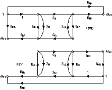
Fig. 1 The signal flow graph for the standard 12-parameter error model with a device under test

This article describes some new calibration methods suitable for three-sampler analyzer calibration. They all provide some of the advantages of self-calibration methods over standard SOLT calibration, either by using fewer calibration standards, or by using a line instead of a matched load.

The standard error model for three-sampler analyzers is the 12-parameter error model, shown in Figure 1, while the standard error model for four-sampler analyzers is a cascade of two error boxes with a total of 7 independent parameters. Since it is not possible to represent a three-sampler analyzer as two cascaded error boxes, a 12-parameter error model must be determined by solving a system of nonlinear equations. The determination of the crosstalk errors E_XF and E_XR is trivial, thus only the determination of the remaining 10 parameters will be described.

TOSL CALIBRATION

The through-open-short-line (TOSL) calibration is a hybrid method, based on both the SOLT calibration and the through-reflect-line (TRL)3 self-calibration method. The supplied reference document provides only approximate solutions.4 An exact solution is given in this article. During calibration, the following need to be measured:

• Open circuit with reflection coefficient Γ₀ (as with SOLT calibration) on both ports. The measurements are denoted M₁₀ on port 1, and M_2O on port 2, as shown in Figure 2 (Equations 1 and 2).
• A short circuit with reflection coefficient Γ₈ (as with SOLT calibration) on both ports. The measurements are denoted M_1S on port 1, and M_2S on port 2 (Equations 3 and 4).
• Through connection (common to both SOLT and TRL calibration) of both ports and S-parameters S_11T = S_22T = 0 and S_12T = S_21T = 1. The raw measurements are denoted M_11T , M_12T M_21T and M_12T as shown in Figure 3 (Equations 5 to 8).
• Calibration line (as with TRL calibration) with propogation constant γ and length l, with the S-parameters S_11L = S_22L = 0 and S_12L = S_21L = e^-γl . The raw measurements are denoted M_11L , M_12L M_21L and M_12L (Equations 9 to 12). Instead of the line, any matched reciprocal two-port element could be used. In such cases, the transmission parameterS₂₁ would appear in the equations in place of the transmission coefficient e^-γl of the line. If the parameters S₁₁ and S₂₂ are known, they can be incorporated into equations 9 to 12.

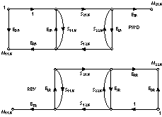
Fig. 2 Signal flow graph of the reflection standards' measurement on both ports of the analyzer; X is either K (known), R (reflect), O (open) or S (short).

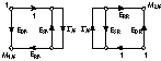
Fig. 3 Signal flow graph of the two-port standard measurement; X is either T (through) or L (line).

The calibration measurements are described by 12 nonlinear scalar equations, which are derived directly from the signal flow graphs by applying the rules for solving flow graphs. Rearranged in a manner convenient for finding their solutions, they are:

Ten parameters of the model are determined from these equations, together with the transmission parameters of the calibration line. One of Equations 7, 8, 11 and 12 is redundant, since the line is a reciprocal element, but due to measurement errors it is beneficial to use all four of them. Similarly, in the TRL method, one of the measurements of the transmission parameters of the calibration line is also redundant, but is usually retained.

The system of Equations 1 to 12 can be solved by iteration. For a first approximation determination, the products E_SF E_LF and E_SR E_LR on the right side of Equations 5 to 12 are set to zero.

Each iteration consists of two steps. In the first step, the values of E_TF and E_TR are determined from Equations 7 and 8, e^γl from Equations 11 and 12 and the two values averaged, E_DF and the product E_RF E_LF from Equations 5 and 9, E_DR and the product E_RR E_LR from Equations 6 and 10.

In the second step, the remaining four linear Equations 1 to 4 are solved for the unknowns E_RF , E_RR , E_SF and E_SR . Finally, parameter E_LF is determined from the E_RF E_LF product, and parameter E_LR from the E_RR E_LR product.

The estimated values of the parameters E_SF , E_LF , E_SR and E_LR from this iteration are then inserted into the right-hand side of Equations 5 to 12, and the whole iteration is repeated. The iteration procedure converges rapidly.

From Equations 5, 6, 9 and 10, it can be observed that e^-2γl must not equal 1; in other words, the length of the calibration line with small losses must not be close to an integer multiple of the half-wavelength. This restriction also applies to TRL calibration, and is one of the weaknesses of this method. The possibility of using a matched attenuator instead of the calibration line is usually mentioned as a way to circumvent this limitation, since with attenuators, the transmission parameter is never equal to 1.

TKRL CALIBRATION

J.A. Jargon et al have proved5 that the following equation is valid for the three-sampler network analyzers:

This relationship consequently means that three-sampler analyzers are completely determined by 11 independent parameters. Therefore, determination actually requires one measurement fewer than with the TOSL calibration previously described. For this reason, in the proposed through-known-reflect-line (TKRL) calibration, one of the reflection standards from TOSL calibration, now denoted as reflect, is not required to be known. Therefore, the following quantities must be measured in addition to through (Equations 5 to 8) and line (Equations 9 to 12):

·         A standard with known reflection coefficient Γ_K on both ports (usually open or short circuits). The measurements are denoted M_1K on port 1, and M_2K on port 2 (Equations 14 and 15).

·         An auxiliary standard with (near) unknown reflection coefficient Γ_R on both ports. Only the approximate phase of the reflection coefficient must be known for this standard, and the measurements are denoted M_1R on port 1, and M_2K on port 2 (Equations 16 to 17).

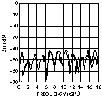
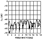
Fig. 4 The absolute value of S₁₁ of the 10 cm MMC 2653 line using TOSL calibration.

The associated equations are

From Equations 5 to 17 (a total of 13, with one of them being redundant for the same reason that applies to TOSL calibration), 10 parameters of the model are determined, together with the reflection coefficient Γ_R , and the transmission parameter of the calibration line.

The equations describing this calibration method are solved by using the same iterative procedure applied in the TKRL method. The first step of the iteration procedure is exactly the same. The second step is somewhat complicated, as the Γ_R reflection coefficient is unknown.

Fig. 5 The absolute value of S₁₁ of the 10 cm MMC 2653 line using TKRL calibration.

In the second step, the remaining five nonlinear Equations 13 to 17 are simultaneously solved for the five unknowns E_RF , E_RR , E_SF , E_SR and Γ_R :

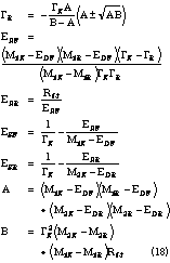
The right side of Equation 13 has been denoted as R₁₃ . The sign in the expression for Γ_R is determined from the approximate value of the phase of this reflection coefficient, which must be known in advance. The product E_RF E_LF determines parameter E_LF , and the product E_VR E_LR determines parameter E_LR . As in TOSL calibration, the length of the calibration line must not be close to an integer multiple of the half-wavelength.

TMKR CALIBRATION

The through-match-known-reflect (TMKR) method is based on through-match-reflect (TMR) calibration.6 It is very similar to the TKRL calibration previously described, the only difference being that a matched load, instead of the calibration line, is measured at both ports. Equations 11 and 12 are now identically zero and 9 and 10 are transformed into:

If the load is not ideally matched, and the reflection coefficient of the load on both ports is known, these values can be used in Equations 19 and 20. There are now 11 equations (Equations 5 to 8, Equations 13 to 17 and Equations 19 to 20) to be solved simultaneously to determine the 10 parameters of the error model and the reflection coefficient Γ_R . The procedure is identical to the procedure for the TKRL method, where E_DF and E_DR are already determined by Equations 19 and 20 and E_RF E_LF and E_RR E_LR are determined from Equations 5 and 6.

VERIFICATION

The systems of nonlinear equations, which define all the proposed calibrations, are well conditioned for real analyzers. Thus, small errors in measurements lead to small errors in the determination of error model. Because absolute values of products E_SF E_LF and E_SR E_LR are small for real analyzers, the result of setting these products to zero in a first approximation is similar to M_L and M_T measured with error. The magnitude of these products for a model HP8720C analyzer is less than 0.03. For this reason, even the first approximation is very good and the iteration procedure converges rapidly. The procedure was also intensively tested by a computer simulation of a three-sampler network analyzer (with or without measuring errors) and the iteration procedure was successful, without exceptions, for all the proposed methods. The procedure was also tested on an HP8720C analyzer and was never at fault.

Verification measurements of the absolute value of S₁₁ of a 10 cm Maury MMC2653 airline are shown in Figures 4 and 5. The measurements have been performed on a three-sampler HP8720C analyzer with APC7 connectors. A Maury model 2650F calibration kit and a 3 cm Maury MMC 2653 reference beadless air-line have been used for calibration. For reference, the same parameters also were measured by using standard SOLT calibration (dashed line).

Fig. 6 The absolute value of S₂₁ of the 10 cm MMC 2653 line using TOSL calibration.

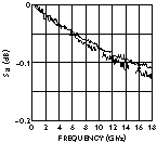
Fig. 7 The absolute value of S₂₁ of the 10 cm MMC 2653 line using TKRL calibration.

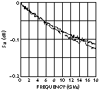
Fig. 8 The phase of S₁₁ of the 10 cm MMC 2653 line using TOSL calibration.

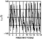
In the vicinity of 0, 5, 10 and 15 MHz (multiples of the half-wavelength of the calibration line), measurements cannot be performed by TOSL and TKRL calibrations, and therefore are missing. Figures 6 to 11 show S₂₁ magnitude and S₁₁ and S₂₁ phase results.

CONCLUSION

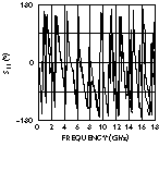
Fig. 9 The phase of S₁₁ of the 10 cm MMC 2653 line using TKRL calibration.

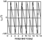
Fig. 10 The phase of S₂₁ of the 10 cm MMC 2653 line using TOSL calibration.

Fig. 11 The phase of S₂₁ of the 10 cm MMC 2653 line using TKRL calibration.

New calibration methods for three-sampler analyzers have been presented. The TOSL calibration method is useful as a direct substitute for the SOLT method for calibrating analyzers with nonstandard connectors, since it is much simpler to manufacture a precise line than a precise matched load.

Since the TKRL calibration is very similar to the TRL calibration, the accuracy of the TKRL calibration is close to TRL calibration, which is considered the most accurate calibration. However, one more reflection standard is required. For this reflection standard, a short circuit that is well defined and can be manufactured precisely for all connectors if not available commercially, is recommended. The same also applies for the proposed TMKR calibration compared with TMR calibration.

ACKNOWLEDGMENTS

The authors wish to thank Radko Osredkar and Matija Kostevc for assistance with the manuscript, and the Dielectric Laboratory of Jozef Stefan Institute, Ljubljana, for providing the measuring equipment.

References

1. J. Fitzpatrick, "Error Models for System Measurement," Microwave Journal, Vol. 21, No. 5, May 1978, pp. 63-66.

2. "New Network Analyzer Offers Choice of TRL Calibrations for Non Coaxial Measurement," HP 8510/8720 News, May 1996, Vol. 7, No. 1, pp. 1-3.

3. G.F. Engen and C.A. Hoer, "Thru-Reflect-Line: An Improved Technique for Calibration the Dual Six-port Automatic Network Analyzer," IEEE Transactions on Microwave Theory and Techniques, Vol. MTT-27, No. 12, December 1979, pp. 987-993.

4. M. Kostevc, J. Mlakar and L. Trontelj, "Calibration TRL for Automatic Network Analyzer with 12 Parameters Error Model," Melecon 85, Madrid 1985, Vol. III, pp. 23-26.

5. J.A. Jargon, R.B. Marks and D.K. Rytting, "Robust SOLT and Alternative Calibrations For Four-sampler Vector Network Analyzers," IEEE Transactions on Microwave Theory and Techniques," Vol. MTT-47, No. 10, October 1999, pp. 2008-2013.

6. H.J. Eul and B. Schiek, "Thru-Match-Reflect: One Result of a Rigorous Theory for De-embedding and Network Analyzer Calibration," 18th European Microwave Conference Proceedings, September 1988, pp. 909-914.

Drago Kostevc received his dipl ing, MS and DSc degrees from the Faculty of Electrical Engineering, University of Ljubljana, Slovenia in 1974, 1981 and 1985, respectively. Upon graduation, he stayed with the University of Ljubljana. The research fields he has worked in include design and modeling of microwave circuits and microwave measurements. Currently, he is an assistant professor of microwave engineering.

Joze Mlakar received his PhD in 1975 from the University of Ljubljana, Faculty of Electrical Engineering. He is currently a professor of electric circuits and electromagnetic waves at the Faculty of Electrical Engineering, University of Ljubljana. His research interests include microwave circuits and measurements and numerical TLM technique for modeling electromagnetic fields.