
Resonator Q, Unloaded/Loaded
For single-frequency oscillators, dielectric resonators placed inside a metallic cavity offer the highest Q and for the frequencies discussed here, resonators with unloaded Q (QU) of 30,000 at 2.856 GHz and 25,000 at 3.9 GHz were obtained.
Coupling to the resonator (loading it) reduces QU to QL and Parker16 established that optimum coupling should occur at S21 = ‐6 dB, where QL =1/2 QU. This coupling factor, leading to QL of 15,000, was used for the 2.856 GHz design. For 3.9 GHz, the reasoning16 was questioned, as 2 dB better PN can be achieved by looser coupling with a resonator insertion loss of 9 dB. The necessary increase in amplification and output power by 3 dB also increases the amplifiers output noise power by 3 dB, but that increase gets suppressed by the resonator’s filtering action. With the above choice, the 3.9 GHz-design was also realized with a QL of 15,000, despite the lower QU.
Amplifier Optimization
The most crucial design decision in the amplifier electronics involves selection of the active device. Here, bipolar silicon transistors are preferred to ensure low fc. Also, designing for high output power pays off, as it lowers the noise floor. Finally, as with all oscillator designs, the device’s transition frequency should be as low as practically possible for building an amplifier with acceptable gain.
That gain has to be some dB above the losses in the loop to accommodate variations over temperature and account for the resonator’s amplitude response over the tuning range. Of course, the occurring gain compression must not lead to instabilities of the amplifier. Low noise device biasing was added to the amplifier design in a two tier regulation scheme that virtually eliminates frequency pushing.
Add-Ons
No oscillator is complete without a buffer amplifier that isolates the oscillator sufficiently from the load. For both designs, double stage buffers were built, reducing pulling to < 1 ppm with a fully reflecting load over all angles, while keeping the noise floor at ‐180 dBc/Hz. Also an ALC was added to stabilize output power to < 0.1 dB, helping reduce phase drifts, due to (tuning induced) amplitude changes.
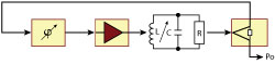
Figure 8 Frequency tuning the transmission oscillator.
Temperature Stability
Frequency tuning of a DRO can be done by either tuning the resonator or varying the phase in the loop (see Figure 8). Most high performance DROs10-13 and the designs presented here provide a coarse mechanical tuning of the resonator (some MHz) and use a phase-shifter (PS) for electronic tuning. Electronic tuning of the resonator, though possible,17 risks degradation of Q as it involves coupling to varactor diodes that have much higher losses.
The available frequency shift from an in-loop PS, however, is confined to a portion of the resonator bandwidth (‐2 dB points in this case). With a QL of 15,000, the tuning range amounts to ±25 ppm. This poses a problem, when the temperature coefficient (TC) of the resonator assembly becomes too high with respect to the targeted temperature range. On top, metallic enclosure (cavity) and dielectric resonator (puck) have different TCs with, even worse, different time responses.12,18
With the aluminium cavity at -1 ppm/K and the 2.856 GHz resonators at +1.5 ppm/K, both TCs cancel well enough, such that this DRO design has no problem to safely operate over a 0°C to 50°C temperature range, more than adequate for the highly temperature controll ed accelerator environments.
The -3 ppm/K TC of the 3.9 GHz resonators, however, adds to the cavity’s TC and allows for just ±6°C of temperature variation that can be compensated with the electronic tuning. As this was felt to be insufficient, a mild sort of oven was incorporated, keeping the assembly at +35°C for long time reliable operation.
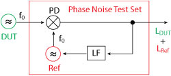
Figure 9 Typical phase noise test setup.
As the problem of temperature drift mounts with rising QL, it will be even more pronounced at lower frequencies (e.g. 1.3 GHz), where QL may increase to 30,000 or more, leaving ±12 ppm or less to be electronically compensated. Meeting this challenge either requires further oven control and thermal insulation or alternative means of electronically tuning the resonator.
Phase Noise Measurement Techniques and Challenges
Measurement of phase noise is a time measurement and as such carried out by comparing two clocks. In addition to the oscillator, or device, under test (DUT), a second oscillator (reference clock) of the same frequency is needed and the time (phase) difference between both oscillators is recorded using a phase detector (PD) (see Figure 9).
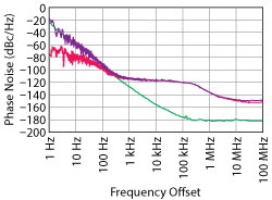
Figure 10 Phase noise measurement of 3.9 GHz DRO with noisy reference.
However, the PD’s output is a measure of the sum of the DUT’s and the reference’s noise power. As long as the reference clock is known to have, say, > 10 dB lower noise than the DUT, the measurement yields a correct result within ±1 dB.
Commercial phase noise test sets19-23 that cover wide frequency ranges, however, incorporate microwave synthesizers as reference clocks. With the phase noise of those synthesizers being decades higher than the phase noise of the oscillators presented here, simple phase detection will not produce the phase noise of the DUT, but rather that of the measurement device’s synthesizer. Figure 10 shows such a measurement (purple trace) that for fm > 300 Hz reproduces the noise of the reference (red trace), whereas the true result of the 3.9 GHz DRO is actually the green trace.
Phase Noise Measurement Using Cross Correlation
A clever way out of this dilemma, enabling phase noise test sets to measure sources with far less noise than their reference has, is the use of a second identical test set, with a second independent reference clock. By letting both test sets measure the DUT simultaneously and combining their outputs by a cross-correlator, it is possible to bring down the noise of the test sets considerably (see Figure 11).

Figure 11 Cross-correlation test setup.
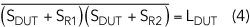
In fact, this cross-correlation technique, that most commercially available phase noise test sets today offer, theoretically, leads to a noise-free test set. The scheme works by transforming the output of the two PDs into the spectral domain (FFT), multiplying them and storing the result. The process is repeated (theoretically forever!) and all stored results are averaged. Mathematically this is represented by:
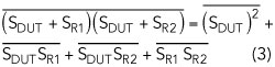
It is important to note that the first term of the right hand side is the phase noise spectral density of the DUT, LDUT. The remaining three terms on the right hand side are called cross-spectral densities, relating two different noise processes and whenever two noise processes are uncorrelated, these quantities are known to be zero.
So in order to build a noise-free phase noise test set, the noise sources nR1 and nR2 in the two test sets must be uncorrelated and the measurement must be carried out forever (ideal averaging requires infinite summations). While the first requirement can be sufficiently fulfilled by sound engineering, the latter requirement is disillusioning, as it ruins the perspective of a noise-free test set in practice.
Yet, the technique is very powerful, as it reduces the test set noise by:
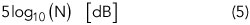
with N the number of cross spectra averaged. So for every 10-fold lengthening of measurement time, 5 dB noise reduction is gained.
It must be stressed that measurement sensitivity with the cross-correlation technique is solely dependent upon measurement time. Most commercial instruments19-23 allow the user to input the number of cross spectra to be averaged as the lever to set sensitivity and measurement time. Less obvious, lowering the start frequency by a decade also lengthens measurement time by a factor of 10 and yields a 5 dB gain in sensitivity. This is because in the time it takes to collect sufficient samples for one correlation in the lowest offset frequency decade (e.g. 1 to 10 Hz), 10x the amount of data is available in the adjacent decade (10 to 100 Hz), allowing 10 cross spectra to be computed and averaged here.
This pattern continues up to the stop frequency of the measurement. Lowering the start frequency by one decade usually has the same effect as increasing the correlations setting by a factor of 10, simply because both steps lead to an increase in measurement time by a factor of 10.