
In communications, noise is an annoying phenomenon. Noise occurs naturally and is random, contrary to human-engineered intelligence. Engineers define the signal-to-noise ratio as the most important quantity that qualifies any information-transmitting system fit or unfit for use.
Researchers utilize sensitive radio and microwave receivers (sometimes also transmitters) to obtain information about various natural phenomena by remote sensing. Noise-like signals emitted, transmitted or reflected by and from various objects can provide interesting data. There are many methods used in remote sensing; some use sensitive receivers-radiometers to detect thermal emission from matter, some can detect non-thermal emission from plasma. In this article, a method of “active” radiometry is introduced, which uses artificial microwave noise as a sounding signal to evaluate both transmission and reflection properties of objects.
 | |||
| Fig. 1 Using a directional coupler to inject a calibrated noise level to a radiometer. | |||
Active Radiometry
Radiometry, in general, is the method of measuring the radiative properties of sources by evaluating the intensity and spectrum of their radiation. This method was first applied in optics, and now extends to the entire known electromagnetic spectrum.
At microwave frequencies, the use of passive radiometry first started in radio astronomy. There, the objects of interest are very remote, like stars and nebulae in the universe. By using radiometric methods, it is possible to determine the temperature of emitting bodies and gases. By analyzing the radiation spectrum, non-thermal effects can also be detected, providing information about magnetic fields and the composition of remote matter.
Passive radiometry has been widely used for remote sensing of terrestrial objects, including the atmosphere, oceans, vegetation and even living bodies. During the development of microwave radiometers for the study of the atmosphere, the radiometer needed to be calibrated by a semiconductor noise source. A directional coupler was necessary to introduce the noise to the receiver input, as shown in Figure 1. More attenuation was then required to adjust the calibration step to a suitable size. The total attenuation rose to more than 60 dB, so the next idea was “what happens if the noise source radiated its noise through open space?”
 | |||
| Fig. 2 Noise source and radiometer with antennas to evaluate the noise field. | |||
As shown in Figure 2, the noise source and the radiometer were separated by one to two feet and provided with small horns. Interesting effects were observed, although similar experiments are familiar to all microwave engineers who use a CW signal.
When using a CW microwave signal, the horns should be separated by at least several wavelengths to avoid the “near zone.” Otherwise, the field intensity filling the close space exhibits strong oscillations that can prevent the experimenter from seeing the small variations due to the radiation pattern of the horn antenna, or, by an object located at the center of a goniometer, as in Figure 3.
 | ||
| Fig. 3 Microwave goniometer to test an object under various angles of incidence. | ||
With the noise source and radiometer arranged as shown, no strong oscillations were observed in the near field — the intensity varied smoothly. Objects placed between the horns caused a loss equal to the value measured with a CW signal, but now the position of the object did not need to be fixed. When slowly moved by hand, the intensity indicated by the radiometer varied by only a small amount, and again, no interference oscillations were observed as with the CW signal. With some improvement in sensitivity, the set up can also measure reflectivity.
As shown in Figure 4, the system, consisting of a noise source and a radiometer, can be used to evaluate an object emissivity, transmittance and reflectance by suitably locating both instruments around the object.7
 | ||
| Fig. 4 Measurements of object properties; (a) loss and emissivity, and (b) reflectivity. | ||
The emissivity is evaluated by sensing the object with the radiometer only; the antenna to be used must be designed so that its radiation pattern is smaller than the object projection (as shown in Figure 5), otherwise a correction must be introduced. The radiometer measures the (noise) temperature of the object and must be calibrated with a “blackbody” of a size greater than the antenna beam and a known temperature. At microwave frequencies, suitable absorbers are available and used as the blackbody.
 | ||
| Fig. 5 Radiometric remote observation. | ||
Next, how the “Active Radiometry” system works is described in detail. The radiometer responds to the noise temperature of the object in accordance with
Txe = E • To (1)
where
E = surface emissivity
To = real temperature of the object
The transmittance, or transmission loss, can be evaluated in two steps: First, the noise source is activated and the radiometer indicates some intensity corresponding to Tn, the noise temperature received from the distant noise radiator. Then the object under test is placed between the noise source and the radiometer. A lower intensity is read at the radiometer output when the noise source is on such that

where
Tn = noise temperature radiated from the noise radiator
The difference between the two readings is proportional to object transmission loss:

 | |||
| Fig. 6 Measuring transmission loss with a variable attenuator in the path. | |||
Using a calibrated attenuator inserted between one of the antennas and the noise source or the radiometer, as in Figure 6, is best because the radiometer output indication can be kept constant. The radiation patterns of the antennas should be smaller than the tested object projection to prevent errors. The arrangement shown previously can be used to evaluate the object reflectivity. With a tested object in place, the radiometer reads
Txr = Tn • R + E • To (4)
where
R = object reflectivity
The reflectivity value can be again assessed with an attenuator, or it is often measured as a percentage of the value obtained from a perfect reflector such as an aluminum screen. Such a screen, and generally all objects, have their reflectivity dependent upon the incidence angle; a goniometer is suitable for such tests.
Noise Radiators
Currently, noise sources use avalanche diodes and their output noise is stable over time and temperature. Such sources, however, must be calibrated for excess noise (temperature) ratio (ENR) as a function of frequency. Calibrating noise sources requires using a wideband sensitive receiver. For instance, the noise source used in the experiments had to be calibrated at 12, 18 and 35 GHz; three radiometers for those frequency bands had to be developed to calibrate the particular noise source. Though the noise diode alone was developed for L-band (VBN 300), the ENR of the noise source was flat from 10 to 20 GHz and the ENR was approximately 30 dB; even at 35 GHz, the ENR was approximately 13 dB.2
Thus, characterizing such wideband noise sources by radiometers is demanding and expensive. It is known in optics, however, that radiation sources can also be evaluated by their coherence.3 The concept of a full coherence means that the radiated wavefront remains a single wave train from the source aperture to a distance named the coherence radius (CR).
For light, lasers exhibit a full coherence up to many wavelengths from a source. At microwaves, a CW signal keeps its coherence at distances such as to the moon and back. Wideband sources and random sources are partially coherent, or incoherent. Their coherence radius is much shorter — the wider the bandwidth, the shorter the CR. Thus, the bandwidth of a noise source could be derived from its coherence radius.
Physicists define the CR as “a distance from a source where the correlation function, or intensity, drops rapidly.”3 As the autocorrelation function of radiation becomes the intensity for zero time delay, the CR was defined as the distance at which the noise-field intensity drops by 3 dB.
Assuming that the noise generator spectrum is roughly rectangular (in the previously described noise source, the waveguide cutoff happened to be at approximately 10 GHz, and a rolloff was expected above 20 GHz), the coherence radius should be2

where
c = speed of light, 3.10E8 m/s
BW = spectrum width in Hz
From Equation 5, the BW can be estimated. By a single CR measurement at 18 GHz (approximately at the center of the generated spectrum), the 3 dB bandwidth was determined to be approximately 10.5 GHz, very close to the 10.67 GHz found by measurement using three radiometers.2
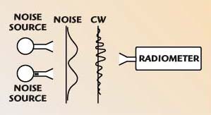 | |||
| Fig. 7 “On screen” response for two noise sources in front of the radiometer. | |||
With two similar noise sources, an equivalent of Young’s interference experiment was done as illustrated in Figure 7. While with coherent (CW) sources an interference wavy pattern of field density is observed, the non-coherent random field results in no interference. By plotting the field density across the screen (by moving the radiometer or the pair of noise radiators), only a smooth rise toward the maximum at the center of each source is observed.
As the noise-field density from each of the two noise radiators causes almost equal radiometer response, the two noise radiators activated together give a field density equal to the sum of both contributions. This was predicted by the Van Cittert-Zernike Theorem4 for coherent and non-coherent optical fields. A matrix of similar noise radiators can be used to create a planar (or curved) noise source with the field density proportional to the number of radiators.
Active Radiometry Applications
The above described method was used to evaluate the emissivity, reflectivity and transmittance of various objects. Its main advantage was observed from the fact that while no anechoic chamber was needed, all tests were easily done on a laboratory bench over distances ranging from approximately 10 to 60 cm.
The microwave noise sources and radiometers were operated at 10, 12 and 18 GHz. Figure 8 provides a method to estimate a maximum loss between a noise source and a radiometer. Three important quantities are shown here — the noise source excess ratio ENR in dB, the radiometer resolution, dT in K, and the maximum attenuation between the noise source and radiometer, L in dB.
 | ||
| Fig. 8 Estimation of measurable loss in a system. | ||
The radiometer resolution or sensitivity, dT, is defined by the minimum discernible step of input noise temperature5 as

where
T = system noise temperature (K)
B = receiver RF/IF bandwidth (Hz)
t = time constant of the radiometer output integrator(s)
 | |||
| Fig. 9 Two designs of noise radiators; (a) an avalanche noise diode, and (b) a SMD transistor. | |||
The above equation is valid for “total-power” radiometers that do not use input noise modulation to separate it from the inherent receiver noise. Using antennas with the noise source and radiometer allows a higher loss L to be achieved, but the effect of the radiation pattern is more important.
Another important feature observed with the use of random fields is that small object movement will not disturb the measurement and usually causes no errors. This feature was used in the design of a sand-moisture measuring system,6 which utilized a simple noise radiator7 and a low cost low noise block (LNB) from a satellite TV receiver. The sand can move freely on a conveyor belt during the measurement, but only a layer not thicker than 2 to 3 cm should be kept for good measurement accuracy.
The noise radiator for a 10 to 12 GHz band can be made as a small half-wavelength dipole with an SMD transistor emitter-base diode in avalanche mode (see Figure 9).6
 | ||
| Fig. 10 Positions of the noise radiator inside the horn (a) and the field density map inside the 20 dB, 10.7 GHz horn (b). | ||
With a noise radiator so small, it became possible to reach inside a microwave antenna structure such as a pyramidal horn (Figure 10), or close to the turns of a helical antenna (Figure 11), or a small parabolic dish, to map the field density distribution and polarization (Figure 12).
Doing such experiments in the near field with CW signals usually requires using an anechoic chamber and processing data with a computer. With noise, it is easy and provides reliable results.
 | ||
| Fig. 11 Field density (in mV) around a 5 turn, 8 mm diameter helical antenna mapped by noise. | ||
 | ||
| Fig. 12 Field density plots on a prime-focus 11 GHz parabolic 1 ft. diameter dish. | ||
Recently, people became concerned with biological effects of electromagnetic fields. The active radiometry uses noise sources emitting microwave power density measured in picowatts per square centimeter, completely negligible compared to CW sources.
To calibrate microwave radiometers, foam or plate absorbers are used as blackbody emitters at ambient or slightly elevated temperatures. It was found that the noise emitted by the described noise source passed through the absorber layer with a loss of 20 to 30 dB. Therefore, a novel design of a “two-level blackbody” was tested, as shown in Figure 13. A noise radiator with a small horn or cavity radiates noise through the blackbody absorber towards the radiometer antenna. Although attenuated, this noise level can be adjusted to add 20 to 50 K, for example, to the ambient temperature of the blackbody, providing the necessary second calibration temperature level.
 | ||
| Fig. 13 Radiometer calibration with a two-level blackbody. | ||
The active radiometry method has also helped in the research of slotted lines, to detect leaky waves predicted in theory, but impossible to detect with CW probing.9 Other devices and procedures using microwave noise can be conceived that utilize the described features of random fields.
Many described experiments were done with the low cost radiometer shown in Figure 14. A low cost, low noise downconverter from a satellite TV receiver is used, followed by a 10 dB IF amplifier and detector. An instrumentation operational amplifier (3/4 LM 324) is used as a DC amplifier with adjustable gain and as an integrator. A 0.5 mA ammeter was used as the output indicator.
 | ||
| Fig. 14 A simple radiometer used with a noise radiator for the described experiments. | ||
Conclusion
A method of active radiometry was introduced in which a noise source and a microwave radiometer are used as replacements to a CW radiator and detector; various experimental observations were described. A substantial advantage was found in that using noise fields makes an anechoic chamber unnecessary and measuring field density in the near-field zone of microwave radiators becomes an easy operation. Some applications of noise field use were presented.
Acknowledgment
The author is indebted to M. Wilson and J. Childers for their valuable comments.
References
- J. Polivka, “Contactless System and Method to Determine Loss and Reflectivity of Objects by Microwave Noise,” Czechoslovak Patent No. AO 260205, 1987.
- J. Polivka, “Active Microwave Radiometry,” International Journal of IR and MM Waves, Vol. 15, March 1995, pp. 1673–1683.
- M. Born and E. Wolf, Principles of Optics, Paragon Press, 1965.
- P.H. Van Cittert, Physica, Vol. 1, 1934, p. 201; F. Zernike, Physica, Vol. 5, 1938, p. 785.
- J.D. Kraus, Radio Astronomy, McGraw-Hill, New York, NY, 1967.
- J. Polivka, “Mapping Field Density Distribution in Microwave Radiators,” International Journal of IR and MM Waves, Vol. 16, October 1996, pp. 1779–1788.
- J. Polivka, “Active Microwave Radiometry in Determining Sand Moisture,” Third Workshop on Electromagnetic Wave Interaction with Water and Moist Substances, April 11–13, 1999, Athens, GA.
- J. Zatocil, Microwave Lab Kutna-Hora, Czech Republic, Private Communication, 2000.
- J. Zehentner, et al., “Spurious Leaky Mode Solutions and Experimental Verification of the Second Leaky Wave,” IEEE International Digest Symposium, April 1999, Anaheim, CA, pp. 1261–1264.
Jiri (George) Polivka received his Ing. and CSc. degrees (MS and PhD degree equivalents) in radio-electronics from the CVUT, Czech Technical University, Prague (now the Czech Republic), in 1966 and 1975, respectively. He worked for the A.S. Popov Research Institute for Radio Communication between 1966–1973, then with the PTT Research Institute, Prague, between 1975–1988, in the areas of microwave technology and wave propagation, and satellite communication technology. He has been a chief scientist with Spacek Labs Inc., Santa Barbara, CA, since 1994. His interests include microwave and millimeter-wave radiometry, including radio-astronomy technology. He can be reached via e-mail at polivka@spaceklabs.com.