
Subsurface prospecting by ground penetrating radar (GPR) is of interest in several applications,1 including civil engineering,2 cultural heritages3 and sub-services detection. A GPR usually works in time domain, transmitting an electromagnetic pulse that, by interacting with the objects buried in the investigated soil, gives rise to backscattered echoes that are gathered by receiving antennas usually in monostatic (transmitting antenna coinciding with receiving antenna) or bistatic (transmitting and receiving antenna spaced by a fixed offset) configurations. By moving the transmitting antenna, a two-dimensional representation of the underground scene (a radargram) can be obtained, wherein the returned signal versus time for each position of the transmitting antenna is represented.1 This strategy is generally sufficient if one only pursues the goal of detecting buried objects. However, if one aims to get additional information in terms of a more accurate localization and extent of the targets, it is useful to have at one’s disposal algorithms able to provide a tomographic image, that is a map of the spatial profile of the dielectric permittivity and/or of the electrical conductivity within the probed buried area.4–5 This can be done by recasting the problem of the subsurface prospecting as an inverse scattering problem, even if this inherently gives rise to ill-posedness and nonlinearity.6
In this framework, the adoption of the simplified linear model provided by the Distorted Born Approximation (DBA)7 allows effective algorithms to be generated, which are needed if the investigation domains are electrically large (which is often the case for subsurface prospecting applications). A linear inversion based on DBA often gives acceptable results (in terms of the localization and of the determination of the geometry of the targets), even in cases where DBA does not hold;8 this is particularly relevant for the applications. Finally, the use of a linear model allows exploiting a powerful mathematical tool as the SVD.9 In fact, SVD allows achieving a stable solution and provides meaningful insight on the spatial variability of the class of retrievable objects.10–13 The solution is obtained by representing the object by means of a finite number of basis functions that depend on the measurement configuration,11 on the properties of the reference scenario5 and on the adopted antennas.14 Therefore, the problem is cast as to search the finite number of parameters represented by the expansion coefficients of the unknown object along the basis functions.
Here, the role played by the excitation law of the transmitting antenna on the reconstruction performances in the framework of a DBA is investigated, based on the inversion algorithm. This is done by analyzing how some properties of the integral relationship, connecting the unknown contrast function and the scattered field that depend on the law of variation of the radiated power versus frequency and locations of the transmitting and receiving antennas. In particular, a simple strategy is explored for a proper choice of the excitation law of the source current in order to improve the performance of the inversion algorithm in extracting information on the low spatial frequencies of the object. The reconstruction of the slower spatial variability of the unknown allows a better localization and reconstruction of the geometry of the object, as will be shown in the following.
The feasibility of the tomographic approach is shown by the reconstruction results obtained by processing in situ measurements, collected during a GPR survey performed in the urban area of Matera (Southern Italy) with the aim of detecting and localizing shallow cavities in the subsoil.
Formulation
The geometry of the problem is given in Figure 1. The upper half-space is made up of air, whereas the homogeneous lower half-space has a relative dielectric permittivity ?b and a conductivity ?b (no magnetic properties are considered).

Fig. 1 Geometry of the problem.
The objects are supposed to have infinite extent along the y-axis, and their cross-section is enclosed in the investigation domain D = [–a, a] X [zmin, zmin + 2b]. The unknowns of the problem are the relative dielectric permittivity ?D (x,z) and the conductivity ?D (x,z) inside the a-priori known investigation domain D.
The source of the incident field is a filamentary y-directed electric current of infinite extent and invariant along the y-axis. The source is multifrequency with a discrete frequency set ranging inside the working band given by ? = [?min, ?max]. The source current is moved along the interface at z = 0 by occupying several abscissas xs within the interval ? = [–xM, xM]. The electric field scattered by the buried objects is measured over the interface at the observation points xo varying also within ?. Therefore, the problem at hand has a two-dimensional geometry and is scalar (the electric field has only a component along the y-axis). A multiview (different locations of the transmitting antenna), multistatic (different locations of the receiving antenna are exploited for a fixed location of the transmitting antenna) and multifrequency (different operating frequencies) configuration is exploited.
In the following, the problem is recast in terms of the unknown “contrast” function, defined as
where

and where

denotes the equivalent dielectric permittivity in the soil. As can be seen, in principle, the contrast function, Equation 1, depends also on the frequency. In this article, such a dependence in the inversion algorithm is neglected (however, the data will take into account this dependence), and a contrast function independent from the frequency is assumed to be an actual unknown of the problem.
Under DBA, which consists of approximating the internal field with the incident field,7 the unknown-data relationship is provided by

where
Es = scattered electric field probed at xo when the source is located at xs
f = frequency
ks = wave-number of the lower half space
Einc = incident field that is the field in absence of the objects and coincides with the field transmitted in the soil
Ge = external Green’s function and gives the field in air radiated by an electric point-source in the soil
By substitution of the expressions of Ge and Einc (given, for instance, in reference 10) in Equation 3, the integral expression of the scattering operator is obtained as
where Io (xs,x0,f) is the level of the excitation current of the filamentary source, and
being the imaginary part of the square root less or equal to zero and ko is the wave-number of the upper half-space (made up of air).
Note that, in Equation 4, the level of the current Io is assumed to vary as a function of the frequency, of the source point and of the observation point. Such a variable current level gives a different “weight” to the scattered field data.
In this article, the attention is focused on the choice of a current law Io(xs, xo, f) that suitably enhances the lower spatial harmonic components of the contrast in the inversion procedure. This can be useful because, in many cases, the most likely buried objects have most of the “energy” of their spectrum concentrated about quite low spatial frequencies.
SVD-Based Analysis
As outlined in the previous section, in order to point out the role of the excitation current, analysis of the retrievable spatial variations of the unknown function is needed. This is made possible by exploiting the SVD tool. The SVD of an operator consists of a triple sequence {un, ?n, vn}: the sequence of the right-hand singular functions un provides an orthonormal basis of the unknown space (in particular of the orthogonal complement to the null space of the operator defined by Equation 3), the sequence of the left-handed singular functions vn provides an orthonormal basis of the data space (in particular of the closure of the range of the operator defined by Equation 3) and the singular values ?n form a non-negative and decreasing sequence of numbers.9
By exploiting the SVD expansion, the formal solution of the inverse problem is given by

where <.,.> labels the scalar product in the data space. In the case at hand, since the kernel of the integral relationship in Equation 4 is an analytic function,15 the singular values have an exponential decay.9 This implies that the solution of Equation 7 must be regularized, and this can be done by truncating the summation in Equation 7 to a finite number N of terms. This provides a truncated SVD (TSVD) solution given by9,16

Equation 8 essentially means that the solution is searched within a finite dimensional space, given by the span of the first N right-hand singular functions un. In order to appreciate some general features of this space, the spectral content function sp is introduced11–13 and defined as

ûm being the double Fourier transform of the mth right-hand singular function um (x,z). This quantity provides an immediate visualization of the filtering properties of the reconstruction algorithm. In fact, since the solution is given by a linear combination of the singular functions above the chosen threshold, the only spatial frequencies that can be retrieved are those where there is a meaningful spatial spectral content. The filtering properties of the operator are correlated with the number N of terms in Equation 8, which depends in its turn on the uncertainties present in the available set of data.9
The spectral content sp, together with the curve of the singular values, can be exploited in order to show the effect of the behavior of the amplitude of the current Io versus the frequency, and source and observation points.
The singular values and the spectral content in the case of a soil having relative permittivity ?b = 9 and electrical conductivity ?b = 0.01 S/m will now be demonstrated. The investigation domain is a square of 1.5 × 1.5 m2 and begins at the depth of 0.1 m. The observation domain ? is a line 2 m long and located at the interface. The sources and the observations are spaced 0.1 m apart, within a multiview, multistatic configuration. The frequencies used are 200, 300 and 400 MHz.
The discretization of the problem is performed by making use of the method of moments (MoM) with point matching in data space. In order to perform the MoM, the unknown is represented with 31 complex harmonic functions along the horizontal direction and 31 step functions along the depth. Figure 2 shows the singular values in the case of a constant Io (solid line). Consider the effect of a variable current source Io. First, the case of a current Io varying only with the frequency will be considered. As stated previously, the aim is to improve the reconstruction of the “slower” spatial variability of the unknown function. To this end, consideration of an excitation law that enhances the value of the current at the lower frequencies is needed. A choice of the excitation law is performed, according to the guideline such that the data must be “potentially of the same relevance.” This means that, in the weighting procedure, the law of variation of the current Io is chosen such that the sub-matrixes relative to the different frequencies used have all the same norm with respect to each other (the Frobenius norm, given by the square root of the sum of the square moduli of the terms of the matrix, is used). It is guaranteed that the comprehensive radiated energy is the same with respect to the Io constant case. In other words, the total radiated power is distributed in a different way but is not changed. In fact, with a constant Io, a higher share of the power would be transmitted on the higher frequencies, while the above redistribution enhances the role of the lower frequencies. The dashed line in the figure depicts the singular behavior in the case of a weighting of the current versus the frequency.

Fig. 2 Behavior of the singular values.
Finally, the case of Io(xs, xo, f) is considered. In this case, Io(xs, xo, f) is chosen such that all the available data have potentially the same weight. This can be numerically performed in a simple way. Since any value of the triple (xs, xo, f) corresponds to a row of the matrix and to a datum, Io(xs, xo, f) is chosen such that the rows of the matrix have the same Euclidean norm. Moreover, the comprehensive radiated power is once again unchanged with respect to the case where Io is constant. The dotted line in the figure depicts the singular values behavior in this last case.
Since the threshold for the TSVD has been fixed at –20 dB (the singular values larger than 0.1 times the maximum singular value in Equation 8 are considered), the dimension N of the space where the solution is searched is the same (N is equal to 90 in each of the three cases at hand). This is due to the criterion adopted in the redistribution of the power, which looks for a reasonable compromise about the “power” of each datum. For example, an indiscriminate increasing of the share of the power radiated at the lowest frequency would surely make the singular value curve much lower, and so the reconstruction would likely be poorer (eventually this would amount to losing the frequency diversity).
However, even if the adopted redistribution of the power has not changed the number of singular values above the chosen threshold, the right-hand singular functions have been modified by the change of the excitation coefficient Io so that the spectral content functions so relative to the three excitation laws are different. They are depicted in Figure 3 in the cases where Io is constant (3a), Io is variable with only frequency (3b) and Io is variable with both frequency and position (3c). In particular, it can be noted that there is an enhancement of the spectral content toward the spatial frequencies, that is those closer to the origin of the spectral domain. This entails an enhancement in the reconstruction of the smoother components of the unknown function and achieves a better localization and determination of the geometry of the object, as will be shown in the following section.

Fig. 3 Spectral contents; (a) Io = constant, (b) Io variable with frequency and (c) Io variable with frequency and position.
Numerical and Experimental Examples
In this section, some reconstruction examples are shown. Numerical results are presented using synthetic data with the aim of outlining the effect of the law of radiated power versus frequency on the features of the reconstructed images. Some results are then given by processing in situ GPR measurements collected in Matera’s San Rocco Square with the aim of detecting and localizing shallow cavities.
Numerical Results
The first test case refers to the reference scenario and the measurement configuration considered in the previous section. In particular, a square object centered with respect to the observation region, sized 0.4 × 0.4 m2, and with relative permittivity equal to 12, and conductivity equal to 0.01 S/m, is considered. Data synthesized within the DBA are exploited (that is, there is no model error on data) and a white gaussian noise is superimposed to the data so that the signal-to-noise ratio (SNR) is equal to 20 dB. The solution is regularized by TSVD with the threshold of the singular values set at –20 dB. The reconstruction of the modulus of the contrast function is shown in Figure 4. In the case of a constant excitation current (4a), the reconstruction of the object agrees to the expectations provided by the spectral content shown previously. In fact, it can be stated that it is possible to retrieve the low spatial variations along the horizontal axis (parallel to the air-soil interface), while for the spatial variations along the depth a band-pass filtering of the inversion scheme is observed. This entails that, for the reconstruction result, it is possible to retrieve the horizontal extent of the object while, due to the band-pass filtering in depth, it is only possible to identify the upper and lower edges of the object.

Fig. 4 Reconstruction with linear noisy data; (a) without weighing of the excitation, (b) weighing of the excitation versus frequency and (c) weighing of the excitation with frequency and position.
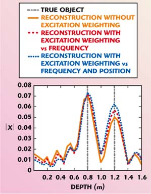
Fig. 5 Behavior of the reconstructions along the central cut of the object..
By passing first to the excitation current variable only with frequency (4b) and then to an excitation current variable with frequency, source point and observation point (4c), an enlargement of the extent of the spectral content can be seen along the lower frequencies in the z direction. This entails that now the reconstruction of the object is improved in particular for the lower edge and the inner part of the object. This can be observed in Figure 5, which depicts the reconstruction in the depth direction along the central cut (at abscissa equal to zero) of the object — the reconstruction is better for the result achieved by weighting the data with frequency and positions. The improvement can be also evaluated in a “quantitative” way by resorting to the correlation index, defined as
where
D = investigation domain
f(x,y) = modulus of the reconstructed contrast function
g(x,y) = characteristic function of the square object (that equals one over the support of the object and zero outside)
The value of the correlation index is at most one when the two functions are proportional to each other (in this case they are “located” on the same support), while it is equal to zero when a complete lack of superposition occurs. Now, in the case at hand, a progressive increase in the correlation index is observed when the conditions pass from the reconstruction without weight (corr = 0.47), to the case of weighting with only the frequency (corr = 0.52) and finally to the case of weighting with the frequency and positions (corr = 0.55).
Finally, an example with data synthesized according to the exact (nonlinear) model of the scattering is shown. An investigation domain of 1.5 × 1.5 m2 that begins at a depth of 0.2 m is considered. The soil is characterized by a relative permittivity ?b = 9 and by a conductivity ?b = 0.02 S/m. An observation region ? of 1.6 m, centered on the investigation domain D, placed at the interface between the two media, is considered. Along the observation region, 17 sources are equally spaced with a spatial step of 10 cm. For each source point, the scattered field is gathered in the same 17 points occupied step by step by the source. The data are gathered at 16 frequencies, equally spaced (with step equal to 20 MHz) between 200 and 500 MHz. A square void 0.4 × 0.4 m2 is considered. The center of the void is at the abscissa 0.4 m, while its depth is 1.3 m. The discretization of the problem is performed by representing the unknown profile in a basis of 37 rectangular pulses along the depth and 37 complex Fourier harmonics in the horizontal direction. The improvement is even more evident than that in the case with model data, probably because the model error due to DBA is lower at lower frequencies.
The synthetic data computed by means of the exact model of the scattering have been corrupted with a Gaussian white noise (SNR = 20 dB). The solution is regularized by TSVD with threshold of the singular values set at –20 dB. Figure 6a depicts the obtained reconstruction corresponding to a constant level I2. The reconstruction with a correction of Io versus only the frequency is shown in Figure 6b, while Figure 6c depicts the reconstruction with a correction of Io versus both frequency, and source and observation positions. A progressive improvement of the reconstruction is observed in terms of the localization of the upper side of the object.
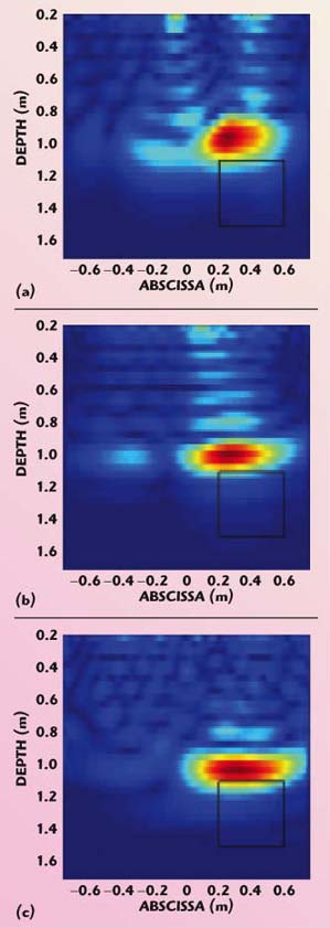
Fig. 6 Reconstruction with nonlinear noisy data; (a) Io = constant, (b) Io varies with frequency and (c) Io varies with frequency and position.
In order to give insight to the practicability of the approach, it is important to show which dynamic range is needed for the transmitter. Figure 7 depicts the relative amplitude of the excitation factor versus the frequency adopted for the reconstruction. The normalization is with respect to the minimum current level, and a natural scale is adopted so that the curve is above the level 1. It can be seen that for the case at hand the required dynamic is limited and does not give a severe constraint about the depth of investigation.

Fig. 7 Behavior of the weighing factor of the excitation versus frequency.
Experimental Results
In this section, some numerical results achieved by the tomographic approach are presented, thanks to the GPR survey performed in the urban area of Matera (Southern Italy). The GPR survey was performed by personnel of the Istituto di Metodologie per l’Analisi Ambientale, CNR with the aim to provide some indication on the causes of unexpected local disarrangement phenomena located inside San Rocco Square. These have created a potential risk condition for the citizens and several problems due both to the stability of the surrounding buildings and to the possible interruption of the crossing road and sub-service networks (sewers, potable water, electricity, telephone, etc.).
The measurements were collected with a GSSI SIR System-2000 acquisition system in time domain with a 200 MHz antenna in a monostatic configuration. The data in the frequency domain was obtained with a fast Fourier transform algorithm. The measurements over two scan lines spaced 2 m apart are used; the overall length of the scan lines is 24 m.
For the tomographic reconstruction, 11 frequencies in the interval 150 to 350 MHz with steps of 20 MHz are used; it can be seen that these frequencies fall within the main lobe of the Fourier transform of the input pulse function. The considered measurement configuration is a multi-monostatic one, and for each reconstruction example a measurement line 3 m wide is considered where the field is collected at 56 points with uniform steps of 5.36 cm.
The investigation domain, where the unknown function is searched, is centered with respect to the observation domain, extends 3 m along the horizontal direction and 1 m along the depth with a minimum depth equal to 0.2 m. In order to achieve a spatial map of the dielectric and conductive properties of the investigation domain, knowing the velocity of the investigating wave is needed (which is dependent on the electrical properties of the host medium). An estimate of the velocity of the investigating wave is determined by measuring the echo-delay time td of a target whose depth z was known as v = z/td, which has provided v = 8 cm/ns in the cases at hand.
With regard to the reconstruction results, the first one refers to an area 3 m long located at the beginning of the first scan line. The reconstruction points out three different anomalies, as depicted in Figure 8. A comparison with a classical radargram is also shown.
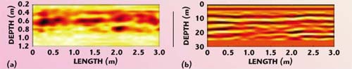
Fig. 8 Comparison between the tomographic image (a) and radargram (b) of the first scan line.
Figure 9 depicts the reconstruction for the investigation domain at the beginning of the second scan line and 3 m long. The corresponding radargram is represented for comparison. It shows a diffuse anomalie more than 2 m wide, which appears as the prolongation of the anomalies present in the first scan line.
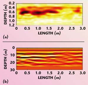
Fig. 9 Comparison between the tomographic image (a) and radargram (b) of the second scan line.
Finally, the reconstruction of the zone between the abscissas 18.5 and 21.5 m (from the beginning of the line, corresponding to the zone of the church of San Rocco) is considered for the second scan line (see Figure 10 ). It points out a diffuse anomaly in the central zone.
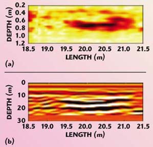
Fig. 10 Comparison of the tomographic image (a) and radargram (b) for the second scan line over a different length.
In spite of the difficult situation (strongly inhomogeneous and quite wet soil, the lack of a particularized characterization of the antennas and of an accurate estimation of the medium dielectric permittivity of the soil), a good correspondence between the tomographic reconstructions and the corresponding radargrams can be seen. The tomographic images, however, seem to show the location of individual anomalies more clearly.
Conclusion
In this article, the effects of the radiated power in inverse scattering from buried objects in the framework of a linear distorted Born-like formulation are investigated numerically. In particular, the role of the law of the source excitation is investigated by means of the SVD tool and guidelines are given in order to enhance the reconstruction of the lower spatial frequencies.
The numerical results show how a suitable choice of the law of excitation improves the reconstruction mainly with regard to the localization and determination of the shape of the object. It is worth noting that the law of excitation can be varied in a very simple way if a stepped frequency GPR is adopted.17
Future developments of this research activity will concern the investigation of the role of the reference scenario (that is, the dielectric and conductive properties of the host medium, possibly also accounting for more realistic dispersion law) and of the antenna’s radiation pattern on a proper choice of the excitation law.
Acknowledgments
The authors thank doctors Vincenzo Lapenna, Vincenzo Rizzo and Sabatino Piscitelli for providing GPR experimental data.
References
- D.J. Daniels, Surface Penetrating Radar, The Institution of Electrical Engineers, London, England, 1996.
- Y.J. Kim, L. Jofre, F. De Flaviis and M.Q. Feng, “Microwave Reflection Tomography Array for Damage Detection in Concrete Structures,” IEEE Transactions on Antennas and Propagation, Vol. 51, 2003, pp. 3022–3032.
- H. Zhou and M. Sato, “Archaeological Investigation in Sendai Castle Using Ground Penetrating Radar,” Archaeological Prospection, Vol. 8, 2001, pp. 1–11.
- G. Leone, R. Persico and R. Solimene, “A Quadratic Model for Electromagnetic Subsurface Prospecting,” AEU International Journal of Electronics and Communications, Vol. 57, No. 1, 2003, pp. 33–46.
- R. Pierri, A. Brancaccio, G. Leone and F. Soldovieri, “Electromagnetic Prospection Via Homogeneous and Inhomogeneous Plane Waves: The Case of an Embedded Slab,” AEU International Journal of Electronics and Communications, Vol. 56, 2002, pp. 11–18.
- D. Colton and R. Kress, Inverse Acoustic and Electromagnetic Scattering Theory, Springer Verlag, 1992.
- W.C. Chew, Waves and Fields in Inhomogeneous Media, IEEE Press, Piscataway, NJ, 1995.
- T.B. Hansen and M. Johansen, “Inversion Scheme for Ground Penetrating Radar that Takes into Account the Planar Air-soil Interface,” IEEE Transactions Geoscience and Remote Sensing, Vol. 38, No. 1, 2000, pp. 496–506.
- M. Bertero and P. Boccacci, Introduction to Inverse Problems in Imaging, Institute of Physics Publishing, Bristol, England and Philadelphia, PA, 1998.
- R. Pierri, G. Leone, F. Soldovieri and R. Persico, “Electromagnetic Inversion for Subsurface Applications Under the Distorted Born Approximation,” Nuovo Cimento, Vol. 24C, No. 2, March–April 2001, pp 245–261.
- G. Leone and F. Soldovieri, “Analysis of the Distorted Born Approximation for Subsurface Reconstruction: Truncation and Uncertainties Effects,” IEEE Transactions Geoscience and Remote Sensing, Vol. 41, No. 1, 2003, pp. 66–74.
- R. Persico and F. Soldovieri, “One-dimensional Inverse Scattering with a Born Model in a Three-layered Medium,” Journal of the Optical Society of America, Pt. A, Vol. 21, No. 1, 2004, pp. 35–45.
- F. Soldovieri and R. Persico, “Reconstruction of an Embedded Slab from Multifrequency Scattered Field Data Under Born Approximation,” IEEE Transactions on Antennas and Propagation.
- F. Soldovieri and R. Persico, “Effects of the Inaccuracy on the Knowledge of Some Parameters in GPR Prospecting,” Remote Sensing in Transition, Millpress, Rotterdam, The Netherlands, 2004, pp. 285–291.
- L.V. Kantorovic and G.P. Akilov, Functional Analysis, Second Edition, Pergamon Press, 1982.
- S. Twomey, Introduction to the Mathematics of Inversion in Remote Sensing and Indirect Measurements, Dover, 1977.
- I.L. Morrow and P. Van Genderen, “Effective Imaging of Buried Objects,” IEEE Transactions on Geoscience and Remote Sensing, Vol. 40, No. 4, 2002, pp. 943–949.