
Linear antennas and their many variations have been essential to wireless communication and sensing for over a century. They have been widely deployed over the electromagnetic spectrum, especially at wavelengths ranging from VLF through microwaves. Even though they have been intensely studied throughout that time, there remain some fundamental questions that affect practical design and performance, and for which the answers are either unresolved, controversial, or mathematically very complicated. They include:
• Does a unique voltage exist along an antenna and, if so, between what easily determined and identifiable points?
• Is there an easy and convenient way to predict the current or voltage standing wave ratio along the antenna more accurately than the zeroth-order approximation of infinity?
• Is there an easy and convenient way to predict the input impedance for monopoles that are odd-integer multiples of a half wavelength (or dipoles that are odd-integer multiples of a full wavelength) more accurately than the zeroth-order approximation of infinity?
In this article, a novel and especially simple mathematical model will be described that provides elegant answers to the above questions and more. While previous investigations have resulted in lengthy and complicated mathematical expressions or computer code, this approach will give rise to remarkably simple formulas. They are also remarkably accurate, providing nearly perfect agreement with far more complicated theories and with measurements.
Perhaps most importantly, this perspective is intuitively appealing and provides a convenient way of thinking about how linear antennas operate as coaxial resonant cavities. This, in turn, should inspire new designs and applications.
Radius of the Virtual Outer Conductor
The investigation begins with the general linear antenna, as shown in Figure 1, where the transverse dimensions are very small compared to a wavelength. The long dimension does not have to be straight and the wire may curve, twist and turn. Further, the transmitter or receiver may be located anywhere along the wire, not just at the center.

Figure 1 The general linear antenna.
In a recent book,1 the author derived a simple but rigorous formula for the characteristic impedance of such a wire that depends only upon its cross-section and the wavelength:

In Equation 1, η is the impedance of free space (approximately 377 Ω) and k’ is the quasi-static wave number:
In Equation 2, γ is Euler’s constant (577215...) and λ is the wavelength.
If Equation 1 is compared with the classic formula for the characteristic impedance of a coaxial transmission line with inner radius a and outer radius b,
Then it is readily found that some sort of equivalent outer radius b for the antenna is:

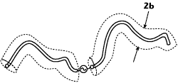
Figure 2 The antenna considered as a virtual coaxial line.
One useful interpretation of Equation 4 is shown in Figure 2. It is seen that the antenna may be conceptualized as a coaxial transmission line with an outer conductor of radius b. That is, b is the radius of a virtual outer conductor for the antenna. This interpretation will lead to many practical formulas and results for actual linear antennas.
An immediate benefit of this interpretation is the answer to the question: “Where and how is the voltage defined along a linear antenna?” With the antenna modeled as a coaxial cavity, the voltage is clearly the potential difference between the inner and outer conductors. That is, the antenna voltage is the potential difference between the actual wire and the virtual outer conductor.
Reflection Coefficient and Standing Wave Ratio

Figure 3 The coaxial resonant cavity terminated by annular slot antenna.
Together with its virtual outer conductor, the antenna may be regarded as a coaxial resonant cavity. Coupling into and out of the cavity occurs at its ends, which are annular slots. Figure 3 shows the details at those ends. On the inner and outer conductors of the coaxial, the forward traveling current has a unity amplitude, and the reflected traveling current has an amplitude Γ. That is, Γ is the reflection coefficient for the current.

Figure 4 A simple circuit representation to calculate the current reflection coefficient.
The circuit representation shown in Figure 4 makes calculation of the reflection coefficient fairly straightforward. In that representation, Rs is the radiation resistance of the annular slot, and Z0 is the characteristic impedance described by Equation 1.
The current in the equivalent circuit is:
When the annular antenna and the coaxial transmission line are matched, then the current is:
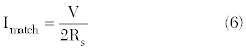
The current I is the superposition of Imatch and a reflected current:

The reflection coefficient is readily found by substituting Equations 5 and 6 into Equation 7 and solving for Γ:
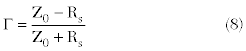
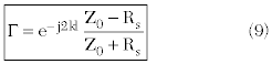
Equation 8 is subtle in at least one way. Close examination shows that it is different from the reflection coefficient obtained using conventional transmission line analysis by a factor of –1. This difference is explained by the unique point of view. The coupling occurs from the annular slot into a coaxial resonant cavity, not the other way around. To transform the reflection coefficient from the plane of the annular slot to the more conventional plane at the input end of the coaxial line, then it must be rotated by a factor of exp (–j2kl), where l is the length of the line:
To evaluate Equation 9, the radiation resistance Rs of the annular slot must first be determined. Since the annular slot is the complement of a wire loop, Booker’s theorem2 can be used.

The radiation resistance of a small loop antenna is:3

Combining Equations 10 and 11, the radiation resistance for the annular slot can be obtained:
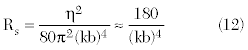
Using the value of b in Equation 4, Equation 12 tells that Rs is approximately 112.5 Ω. The current or voltage standing wave ratio is defined as:

Applying Equation 9 to Equation 13, the surprisingly simple formula can be obtained:
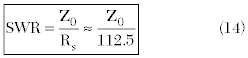
Figure 5 shows the standing wave ratio for a wide range of practical antenna characteristic impedances.

Figure 5 Voltage or current standing wave ratio along a monopole antenna as a function of its characteristic impedance.
Input Current and Input Reactance
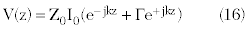
The current and voltage inside the coaxial resonant cavity can be easily written down using the reflection coefficient determined as in Equation 9. If z is the longitudinal coordinate along the cavity, then the current is described by the usual transmission line formula:

The choice of the minus sign with the reflection coefficient Γ is consistent with the discussion of the previous section, and with Figures 3 and 4 in particular.
The voltage, or potential difference between the inner and outer conductors, is:
The impedance along the line is:

Equations 15 to 17 will provide convenient formulas for the input current and input reactance. The current is:


Figure 6 Input current magnitude for monopole antennas of different lengths, and of different characteristic impedances.
Figure 6 shows the results of evaluating Equation 18 for antennas of varying lengths and characteristic impedances. It is seen that the current never quite vanishes, although its minima decrease monotonically with increasing characteristic impedance. This is in agreement with intuition. Further, the formula answers the question: “What is the value of the input current for monopoles (or dipoles) that are an odd-integer number of half-wavelengths (or full wavelengths for dipoles), more useful and with better accuracy than the zeroth-order approximation of zero?”
The input reactance is:
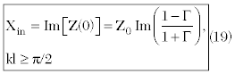
For short antennas, the classic open-circuited transmission line model is more convenient:

Equations 19 and 20 agree with each other exactly for kl= π/2.
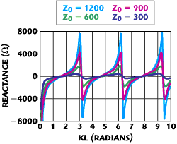
Figure 7 Input reactance for monopole antennas of different lengths, and of different characteristic impedances.
Figure 7 shows the input reactance for antennas of varying length and for various characteristic impedances using Equations 19 and 20. It is seen that its magnitude is large for odd-integer half-wavelength monopoles, and zero for even-integer half-wavelengths. Again, the model answers the question: “What is the value of the input reactance for monopoles (or dipoles) that are odd-integer number of half-wavelengths (or full wavelengths for dipoles), more useful and with better accuracy than the zeroth-order approximation of infinity?”
Radiated Field and Input Radiation Resistance
The current distribution described by Equation 15 readily determines the radiated electric field:4

In Equation 21, the vertical radiation characteristic is:

Equations 21 and 22 describe the contributions to the radiated electric field from z-directed currents. Similar formulas describe any contributions from wires bent in the x or y directions. For simplicity, here the examples will be limited to vertical, or z-directed antennas. For such geometries, Equation 22 can be evaluated exactly in terms of simple functions;5 however, with modern desktop computers, it is quickly evaluated numerically as well.
From the radiated electric field, the radiated power density, or Poynting vector, is readily obtained:

And also the total radiated power:

For vertical or z-directed wires, using Equations 21 to 23, Equation 24 becomes:
Finally, the input radiation resistance is:

Equation 18 is used to compute Iin in Equation 26.
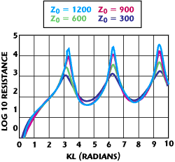
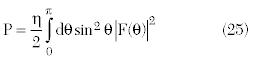
Figure 8 Input resistance for monopole antennas of different lengths, and of different characteristic impedances.
Figure 8 shows the input radiation resistance for antennas of varying lengths and characteristic impedances, computed using Equation 26. It is seen that it is very large for monopoles that are an odd-integer number of half-wavelengths, and that value increases monotonically with increasing characteristic impedance. Again, the model answers the question: “What is the value of the input resistance for monopoles (or dipoles) that are odd-integer number of half-wavelengths (or full wavelengths for dipoles), more useful and with better accuracy than the zeroth-order approximation of infinity?”
Comparison with Measurements and with Other Theories
The most sensitive (in the sense that they are highly variable) and historically controversial results are the ones described in the previous section, namely, the value of input resistance for monopoles that resonate at an odd-integer number of half-wavelengths. These values are typically orders of magnitude greater than the input resistance of antennas with non resonant lengths. Perhaps surprisingly, the results of the simple model agree almost exactly with both measured results and those of much more complicated theories.
Figure 9 The input resistance of a half-wave monopole as a function of characteristic impedance.
Figure 9 shows the input resistance for half-wave monopoles as a function of characteristic impedance. A few data points from the classic reference by Sergei A. Schelkunoff6 are plotted in the same figure. These data points represent both measurements and Schelkunoff’s mathematical model. The latter is very complicated compared with the model proposed and involves lengthy expressions of higher transcendental functions such as sine integrals and cosine integrals. The agreement is close if not exact within the ability to precisely read data from the figure in Schelkunoff’s book.
Effect of End capacitance and Top Loading
For many, if not most, practical antennas, the reflection coefficient described by Equation 9 is perfectly accurate. There are some exceptions, however, especially for antennas with actual radii that are significant fractions of a wavelength. For those antennas, the end termination is not only an annular slot but also a disk capacitor. The reactance of that capacitor is easily included in the model.
There is a classic formula for the capacitance of a single disk in free space:7

where ε is the permittivity of free space, approximately 8.854 pF/meter.
In the case of top loading, the capacitance is deliberately increased by modifying the end of the antenna, typically with guy wires or other improvised conducting surfaces.
Whether the capacitor is simply the intrinsic disk or a carefully designed enhancement, its reactance is:
To improve the accuracy of Equation 9 for the reflection coefficient, the reactance must be put in parallel with the slot radiation resistance. This creates a new, complex load impedance:
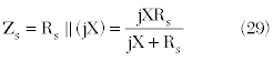
Using Equation 29, Equation 9 is replaced by:


Figure 10 The effect of end capacitance and top loading on the input resistance of a half-wave monopole.
Figure 10 shows the effect of disk capacitance or top loading on the input resistance of resonant, half-wave monopoles for varying characteristic impedance. This figure is the same as the preceding one, with the results modified by using Equation 30 instead of Equation 9. Significant effects are seen for reactances X with magnitudes comparable to or smaller than the slot radiation resistance Rs. As X increases in magnitude, however, the effect vanishes, as expected.
Conclusion
A simple formula for the characteristic impedance of a single cylinder or wire has led to a comprehensive yet mathematically simple model for a vast family of antennas. That family includes all monopoles, dipoles and other linear antennas. It also includes multi-conductor antennas and antennas with non-circular cross-sections that can be reduced to a single wire with an equivalent radius.8 The model provides simple formulas that answer practical, but difficult design questions concerning the standing wave ratios, input current and input impedance of antennas, especially at resonant wavelengths. Previously, long and complicated mathematical expressions were required to get at those answers. The answers given here agree almost exactly with those complicated expressions and with experimental measurements. The model also provides a novel and convenient point of view regarding linear antennas. That is, they are coaxial resonant cavities. Coupling into and out of the cavity occurs at the ends via an annular slot. For top loaded antennas and for antennas with radii not small compared with a wavelength, a capacitor is connected in parallel with the slot.
References
1. J.K. Raines, Folded Unipole Antennas: Theory and Applications, McGraw-Hill, New York, NY, 2007, pp. 225-232.
2. H.G. Booker, “Slot Aerials and Their Relation to Complementary Wire Aerials (Babinet’s Principle),” Proceedings of the IEEE, Part IIIA, Vol. 90, No. 4, April 1946, pp. 620-626.
3. E.A. Wolff, Antenna Analysis, John Wiley & Sons Inc., Hoboken, NJ, 1966, p. 77.
4. Ibid, p. 39.
5. J.K. Raines, Folded Unipole Antennas: Theory and Applications, McGraw-Hill, New York, NY, 2007, p. 45.
6. S.A. Schelkunoff and H.T. Friis, Antennas: Theory and Practice, McGraw-Hill, New York, NY, 1952, p. 441.
7. M. Mason and W. Weaver, The Electromagnetic Field, University of Chicago Press, Chicago, IL, 1929; reprinted by Dover Publications, p. 133.
8. J.K. Raines, Folded Unipole Antennas: Theory and Applications, McGraw-Hill, New York, NY, 2007, pp. 245-248.
 Jeremy Keith Raines received his BS degree in electrical science and engineering from MIT, his MS degree in applied physics from Harvard University and his PhD degree in electromagnetics from MIT. He is a registered professional engineer in the state of Maryland. Since 1972, he has been a consulting engineer in electromagnetics. His antenna designs span the spectrum from ELF through SHF. He may be contacted at www.rainesengineering.com.