
Measuring far field antenna patterns requires separating the transmit antenna and the antenna under test (AUT) by a large distance in order to minimize the field amplitude and phase variations across the test aperture. When the AUT is many wavelengths across, the far field distance becomes quite large. Thus, in order to measure the antenna pattern of an electrically large aperture indoors, techniques like a compact range, near field scanning and antenna focusing are necessary. These approaches allow for accurate prediction of the far field pattern even though the measurements are taken in the near field. The field variations across the AUT become smaller as the separation distance increases.
The IEEE defines the far field of an AUT in terms of the maximum phase deviation across the AUT. For non-low sidelobe antennas the maximum phase variation is  /8 radians, and the corresponding far field distance is defined by

where
D = the maximum extent of the aperture
 = the wavelength
The greatest phase variation for a rectangular aperture occurs at one of the corners, and D is the diagonal of the AUT. As D gets large and/or gets small, the minimum Rff increases. The phase and amplitude variations across the AUT are highly correlated. These correlated variations result in pattern variations close to the main beam; far from the main beam, however, the pattern is relatively undisturbed.1
Antenna arrays have been used to generate a planar field in a test volume for electromagnetic susceptibility testing. Hill used a constrained least squares approach developed by Mautz3 to create an approximate plane wave in the near field. The results show a reasonably flat (within 3 dB) amplitude response for small linear arrays of line sources. The phase response is not shown and implementing the source constraint is limited. This approach was experimentally applied to a seven-element array of Yagi-Uda antennas at 500 MHz.4 The results were very encouraging. In another study, a circular array was synthesized to create a plane wave at the interior of the array elements.5 Scanning of the plane wave is demonstrated. For further background information on creating a plane wave in the near field, the reader is referred to J.E. Hansen.6
A more recent method was developed to create a plane wave in the near field from a linear array of line sources7,8 using a genetic algorithm. This approach combines the ideas of array focusing and a compact range. The location and weights of an array of line sources were found that approximate a plane wave at a desired location in space. The optimized amplitude and phase ripples across the AUT are much less than those created by a uniform array with the same number of elements. The optimized approximate plane wave is a significant improvement over a uniform array or a single line source. This method also proved successful in experimental testing, as reported in Courtney, et al.9,10 The idea behind these papers is to find the amplitude, phase and position of the elements that create a relatively constant field amplitude and phase along a linear aperture in the near field. A linear array can only control the field in the plane of the array but not the field in the orthogonal plane. The resulting plane wave is robust in bandwidth and physical depth.8
This article presents results of generating a plane wave using a planar array instead of a linear array. The complex array weights are found using a least square solution and compared to the results found using a genetic algorithm. This technique significantly reduces the separation distance between the transmit antenna and the AUT.
Formulation
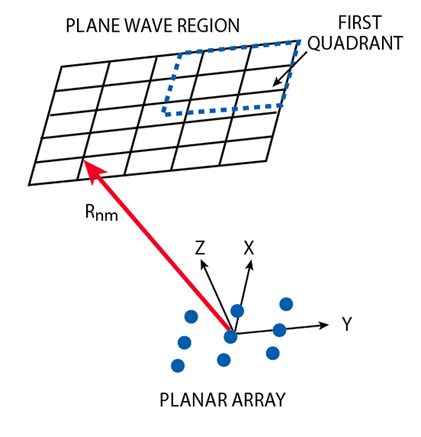
The mathematical expression for the transmit planar array of isotropic point sources shown in Figure 1 is given by

where
Nel = number of elements in the array
wn = anejpn = complex weight of element n
k = 2 /
= wavelength
Rmn = distance from element n to the field point (xm,ym,z0) on the plane wave
z0 = distance from array to the plane wave
The 1/Rmn factor produces small amplitude deviations across the desired plane wave area some distance from the array. On the other hand, the exponential factor creates large amplitude and phase deviations across that same planar area. The planar array lies in the x-y plane; the plane wave region is also in the x-y plane but z0 away from the array. The array elements are in a square lattice. Samples in the plane wave region are also on a square grid.
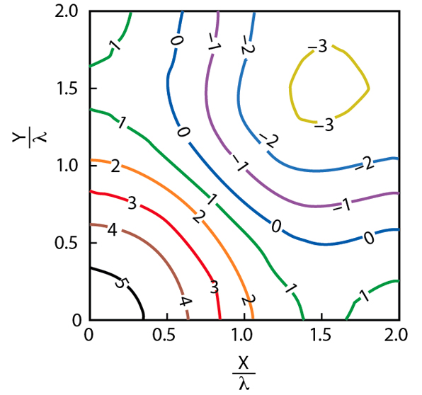
Consider a 6 x 6 element transmitting array with elements arranged in a square lattice with spacings dx = 1.0 and dy = 1.0 . These large spacings reduce mutual coupling effects, making the point source model a better approximation to reality. Optimized spacings previously reported7 were on the order of a wavelength or larger. The desired 4 x 4 l plane wave region is z0 = 10 away from the transmitting array. This distance is considerably less than the far field distance of Rff = 64 . Moving this plane wave region to Rff = 64 would result in a phase variation of 22.5° and amplitude variation of 0.33 dB. If the array weights are uniform, then the amplitude distribution at the plane wave region is shown in Figure 2 and the phase distribution in Figure 3 . These plots are the first quadrant of the plane wave region with the other three quadrants being symmetric about the x- and y-axes. The point (0,0) is the center of the plane wave region and is where the four quadrants meet. The maximum phase variation across the plane wave region is 60° and the maximum amplitude variation is 8.6 dB. These variations far exceed the IEEE standard and are unacceptable for most measurements. The next two sections present two approaches to minimizing the amplitude and phase variations in the desired plane wave region.

Approach I: Least Squares
Equation 2 can be put in matrix form Ax=b, where A is the Green's function matrix, x the complex element weights and b the field values at the plane wave. The resulting matrix equation is given by

When M = N, a direct solution is found; otherwise, when M > N (more field points than elements), a least squares solution is found. Since the exact field values at the plane wave are unknown, the amplitude is assumed to be one and the phase zero. Once the weights are found, they are normalized.
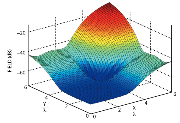
Solving Equation 3 (given the same array configuration as in the last section) yields weights that produce a very flat amplitude and phase field distribution over the plane wave region. In fact, using M = 81 sample points in the quadrant results in weights that produce a maximum amplitude variation across the plane wave region of 0.003 dB and a phase variation of 0.02°. These amazing results are at a cost, though. Unfortunately, the plane wave has extremely low amplitude as can be seen in a plot of the expanded region about the desired plane wave, as shown in Figure 4 . Note the very flat amplitude response in the desired plane wave region; the level is at approximately -70 dB compared to the +5 dB for the uniform array. This very low level would place the plane wave in the noise level of an experimental setup. The low amplitude, coupled with significant scattering from nearby objects illuminated with high amplitude fields, makes this approach impractical.
The plane wave appears at such a low level because half the array weights are out of phase with the other half; in other words, it is a difference pattern with a null in the main beam. In the far field, the 1/Rmn terms are replaced by a constant 1/R that can be factored out of the summation. In addition, symmetry can be imposed on both the amplitude and phase of the array weights in the form of combining symmetric phase terms using Euler's identity for cosine. In the near field, however, Rmn is not a constant and the amplitude of symmetric phase terms are not the same, so symmetry cannot be imposed. Consequently, numerical optimization must be used to find an acceptable solution.
The least square constraint originally proposed in Mautz3 and used to generate near field plane waves in Hill2 was tried. It requires the source weights to have the constraint

where C is a constant. Unfortunately, the Green's function matrix has a large condition number (on the order of 1010), so when the Hermitian matrix is formed from the Green's function matrix (see the procedure in Mautz3 and Hill4), the condition number is even higher (on the order of 1017). This condition number invalidates any results obtained with double precision arithmetic. Thus, another approach is needed for this planar array configuration.
Approach II: Genetic Algorithm
This optimization problem is of sufficient complexity that a local optimization algorithm, such as the Nelder Mead down-hill simplex or conjugate gradient, does not find an adequate solution. Consequently, a GA is used to explore the multi-modal landscape of the cost function. One advantage of the GA is the ease with which constraints are added to variables. In this case, the array weights are bound by 0 
 n 1 and 0 Pn 2 . Analytical-based methods like least squares require an extensive effort to add constraints and the constraints are very limited. The GA also does not have to worry about the condition number of the Green's function matrix. In addition, imposing symmetry on the array weights about the x-axis and y-axis eliminates the possibility of creating the plane wave in a null of the field pattern. Unlike least squares, the GA can also optimize array element spacing in all directions and can be used with experimental data. Thus, the GA could be used in the actual experimental setup and adjusted for environmental effects.
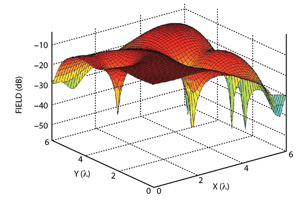
The objective function used in this minimization is given by
where Em are the complex field samples from the desired plane wave region. Values of the objective function, or cost, generally range between 0 and 2. The first term is the maximum phase deviation normalized to . As long as the plane wave area is not too large, this term stays less than one. The second term is the normalized maximum field amplitude. These terms can be weighted to achieve a desired emphasis on either the field amplitude or phase. In this example, they are weighted equally.
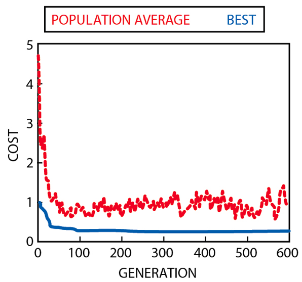
The continuous parameter GA used a population size of 80 with 1 percent mutation rate, 50 percent crossover rate, single point crossover, and ran for 30,008 function evaluations. Figure 5 shows the GA's progress over 600 generations. Most of the work was completed in about 40 generations and the result was essentially attained in less than 100 generations. The solid line is the best cost in the population at each generation, while the dashed line is the average cost of the population of 80 chromosomes. Fluctuations in the average population cost are due to mutations.
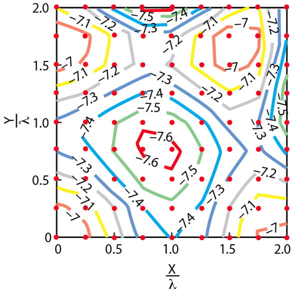
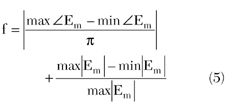
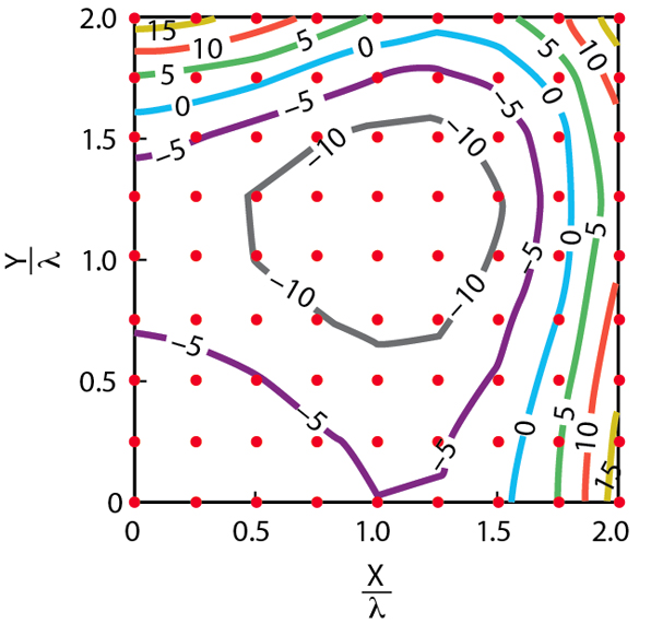
The results are quite good. The maximum field amplitude variation across the desired plane wave region is 0.75 dB, as seen in the contour plot of Figure 6 . The maximum field phase variation across the desired plane wave region is 32.4°, as seen in the contour plot of Figure 7 . These field variations are a significant improvement over the same field variations due to a uniform array. The field amplitude is 60 dB higher than the least squares solution. Figure 8 is a plot of the field amplitude over an extended area about a quadrant of the plane wave. Unlike the field amplitude resulting from the least squares approach, this amplitude drops off outside the 2 x 2 plane wave quadrant. Table 1 displays the optimum array weights found by the GA.
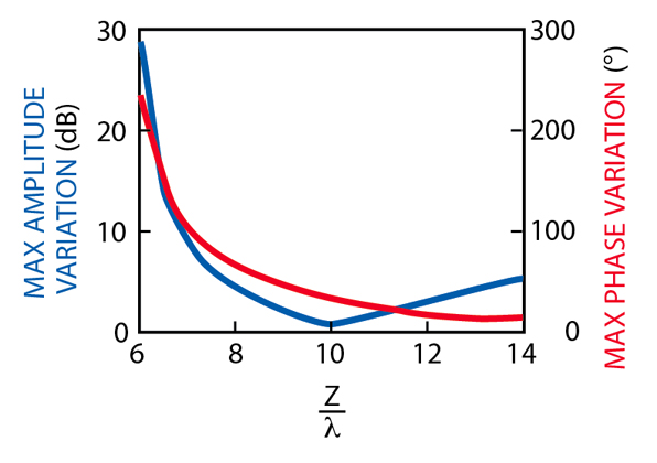
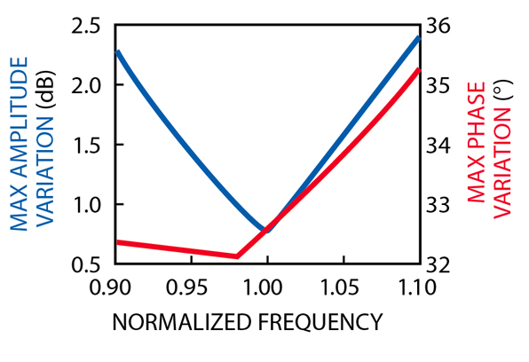
It is important to investigate the sensitivity of the optimization result to changes in separation distance or frequency. The array weights were optimized for a frequency of f0 and a separation of z0 = 10 . Figure 9 shows the maximum amplitude and phase variations over the plane wave region as a result of moving the transmit array in z. The greatest harm to the plane wave is done by decreasing the separation distance, because both the amplitude and phase variations increase. Increasing the separation distance produces greater amplitude variations but less phase variations. The decrease in phase variations results from z0 moving closer to the far field. These results indicate that the separation distance in an experimental setup at 1 GHz could be a few centimeters in error without much impact on the plane wave. Figure 10 shows the maximum amplitude and phase variations over the plane wave region as a result of changing the frequency, f0. The maximum deviations are much sharper for changes in frequency. There is a clear minimum for maximum amplitude deviations at f0. The minimum of the maximum phase deviations occurs at 0.98f0. Phase variations increase above the center frequency because the far field distance Equation 1 increases as the wavelength decreases. If testing occurs over a bandwidth, then the optimization should be done at the highest frequency instead of the center frequency.
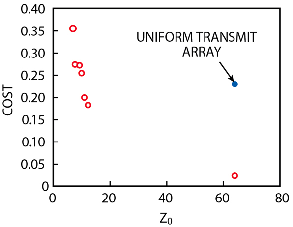
Many different optimization runs were done for various transmit antenna configurations, separation distances and plane wave region sizes. Good results were obtained for element spacings between 0.5 and 1.5 . Increasing the plane wave size or decreasing the separation distances increases the field variations across the desired plane wave region. Figure 11 is a graph of the best cost found by a GA for the 4 x 4 plane wave region at a distance given by z0. A single point for the uniform transmit array is plotted at z0 = 64 for comparison. Figure 12 is a plot of the optimized cost vs. the width of the plane wave at z0 = 10 . If the transmit antenna were a linear array, then the maximum extent of the plane wave region would be 4 . Since the plane wave region is square, the maximum extent is a diagonal that is 5.7 wide. There is a trade-off between field amplitude and phase variations that can be exploited by weighting the terms in the cost function. Thus, a smoother field amplitude is possible at the expense of more variations in the field phase, or visa versa.
Conclusion
This article presents a new way of generating an approximate plane wave region in the near field using a planar array. Previous approaches used only a linear array. A least squares approach produces an impractical implementation. Adding a constraint to the least squares solution raises the condition number of the Green's function matrix to an unacceptable level. The GA design produces an approximate plane wave with small amplitude and phase variations. It is possible to increase the separation between the transmit array and the approximate plane wave region without much decrease in performance. Decreasing the separation distance, however, dramatically increases the amplitude and phase variations. The amplitude and phase variations increase as the frequency moves away from the design center frequency. Increasing the frequency increases the variations more than decreasing the frequency.
Although this problem was modeled with isotropic point sources, the GA works with any form of cost data. This data can be in the form of the output from a mathematical function or an experimental measurement. As such, the point sources could be replaced by better antenna models or experimental measurements and the GA would still find an optimal solution. When the idealized point sources in references 7 and 8 were replaced by an actual experiment in references 9 and 10, the GA was found to produce comparable results.
References
1. E. Brookner, Practical Phased Array Antenna Systems, Part 2 , "Antenna Array Fundamentals," Artech House Inc., Norwood, MA 1991.
2. D.A. Hill, "A Numerical Method for Near-field Array Synthesis," IEEE Transactions on Electromagnetic Compatibility , Vol. 27, No. 4, November 1985, pp. 201-211.
3. J.R. Mautz, "Computational Methods for Antenna Pattern Synthesis," IEEE Transactions on Antennas and Propagation , Vol. 23, No. 4, July 1975, pp. 507-512.
4. D.A. Hill, "A Near-field Array of Yagi-Uda Antennas for Electromagnetic-susceptibility Testing," IEEE Transactions on Electromagnetic Compatibility , Vol. 28, No. 4, August 1986, pp. 170-178.
5. D.A. Hill, "A Circular Array for Plane-wave Synthesis," IEEE Transactions on Electromagnetic Compatibility , Vol. 30, No. 1, February 1988, pp. 3-8.
6. J.E. Hansen, Spherical Near-field Antenna Measurements , Chapter 7, "Plane-wave Synthesis," Peter Peregrinus Ltd., London, England 1988.
7. R.L. Haupt, "Generating Plane Waves from a Linear Array of Line Sources," Antenna Measurement Techniques Association Conference , Denver, CO, October 2001.
8. R.L. Haupt, "Generating a Plane Wave with a Linear Array of Line Sources," accepted for publication in IEEE Transactions on Antennas and Propagation .
9. C.C. Courtney, D.E. Voss, R. Haupt and L. LeDuc, "The Theory and Architecture of a Plane-wave Generator," Antenna Measurement Techniques Association Conference , Cleveland, OH, November 2002.
10. C.C. Courtney, D.E. Voss, R. Haupt and L. LeDuc, "The Measured Performance of a Plane-wave Generator Prototype," Antenna Measurement Techniques Association Conference , Cleveland, OH, November 2002.

 Randy Haupt received his BS degree in electrical engineering from the USAF Academy, his MS degree in electrical engineering from Northeastern University, his MS degree in engineering management from Western New England College and his PhD degree in electrical engineering from the University of Michigan. He is currently a professor and the head of the electrical and computer engineering department at Utah State University. His research interests include genetic algorithms, antennas, radar, numerical methods, signal processing, fractals and chaos. He has published numerous journal articles, conference publications and book chapters on antennas, radar cross-section and numerical methods, and is co-author of Practical Genetic Algorithms (John Wiley & Sons Inc., New York, NY 1998). Haupt has eight patents in antenna technology and is director of the USU Anderson Wireless Center.