In the previous two blogs, I have discussed the architecture difference between swept and stepped analyzers, and some of the subtle differences in stepped analyzers including real-time analyzers.

This has developed some of the important figures of merit when considering the use of a spectrum analyzer: speed, dynamic range, bandwidth, and minimum event duration for 100% probability of intercept.

Now let’s look at the exact same signal on each of the different architectures and describe the differences in the observed signal.  The signal of interest is a frequency hopping signal that dwells at three separate frequencies a couple MHz apart at a carrier frequency around 2.4 GHz.  The signal tunes, overshoots, settles, and dwells at each frequency for all in about 400 us before sequentially changing to the next frequency in a repetitive pattern.  Thus, there are about 2500 transitions per second.

The span and resolution bandwidth are held constant between the three different architectures:  20 MHz Span, 20 kHz RBW.

Swept Analysis

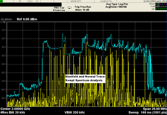
Figure 1.  The swept analyzer architecture

As shown in Figure 1, the swept architecture takes 146 ms to sweep across 20 MHz in a 20 kHz RBW.  During this swept time, there are 100’s of transitions and dwells.  Because the analyzer is sweeping, and the RBW limits the observable bandwidth, spectral events are represented as single narrowband amplitude events.  Using the maximum hold trace, you can collect andobserve a signal over a period of time and get a rough view of the overall bandwidth the signals occupy.  However, the signal behavior is hardly visible or intuitive from the spectrum display for this type of signal.

Time overview not possible at the same time you are viewing the spectrum, but a time overview will only show you the amplitude vs time within the RBW setting.  This signal might not be changing amplitude, but it is changing frequency.

Stepped – Vector Signal Analysis

Since the stepped analyzer has the ability to see the entire bandwidth of the signal in the IF, the vector analyzer shown in Figure 2a below allows you to see the Frequency vs Time and the Spectrum at the same time for this signal.  The horizontal time domain display is set to 200us/division, and the frequency vs time trace shows the frequencies and transitions of the signal of interest for an entire sequence.

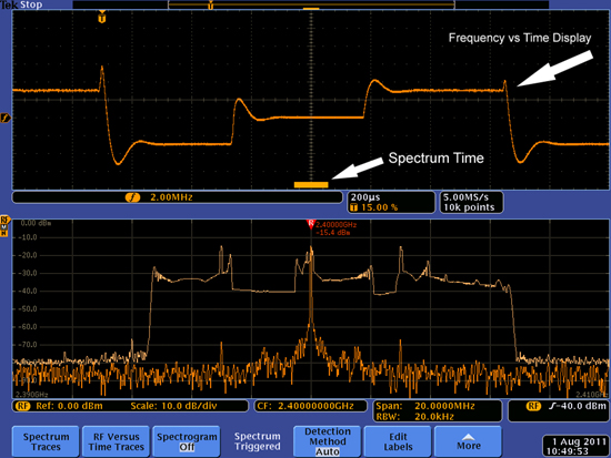
Figure 2a.  A vector signal analysis FFT computed during a dwell period.

With the flexibility to view the time-domain behavior of the signal and the frequency-domain behavior, now comes the requirement to show the correlation between the domains.  The Spectrum Time shows the acquisition time required to compute the correlated spectrum display.  At a 20 kHz RBW (Kaiser Window), the acquisition time associated with the spectrum calculation is about 112 us.  This is over 1000 times faster than the sweep of the spectrum analyzer across the same span.

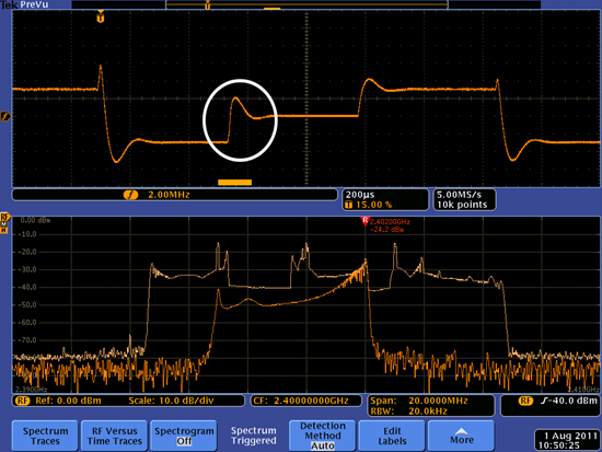
Figure 2b.  Spectrum time observed during fast transition

Looking at the spectrum during the frequency transition between low frequency and the middle frequency of the three hops, Figure 2b, the FFT smears across the spectrum due to the changing frequency during the spectrum acquisition.  This is an expected artifact, and can help explain the spectrum energy of the swept analysis of figure 1.  The smeared spectrum would be represented by a signal tone at the frequency of the sweep generator on the spectrum analyzer due to the very slow observation period relative to an FFT.

Stepped -  Real-time Analysis

The real-time analyzer is based on vector signal analysis technology, so it also allows the time-domain and frequency-domain views of a signal to be observed.  In addition to the vector analysis capabilitity, the real-time processing engine in the analyzer enables a continuous and persistent view of the spectrum display.

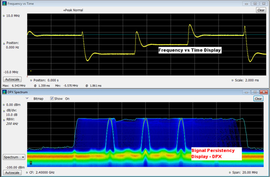
Figure 3. The Real-time Analyzer can show the long-term persistency of the signal.

Figure 3 shows a color graded temperature scale of the persistency display (DPX).  Red colors, like the noise, occur most often, while blue occur infrequently.  It is instantly observed in the persistency display that this signal appears to have three quasi-stable states at three different frequencies.  It is also easily seen using the MaxHold trace on the DPX display (green trace), that the observed spectrum is actually at a higher level than what has been observed on the swept analyzer and the vector signal analyzer.

This last part relates to the Probability of Intercept and the ability of the real-time analyzer to see all the spectrum signals for very fast events.  The minimum event duration is as fast as 3.7us. 

It is clear that the other analyzers did not see these during the time spent observing the signal.  Perhaps if we left the other analyzers on MaxHold for a couple hours, the results would be closer.  Personally, I’m not that patient.