

The microstrip interdigital filter design is very sensitive to the absolute placement of the resonator grounding vias and the alignment of the metal pattern to the vias. It is easy to imagine a somewhat random distribution of resonant frequencies in the etched filter. Measured data for the 3.5 GHz filter can be found in Figure 18 (a), along with the simulation results, while the same data for the 5.8 GHz filter can be found in Figure 18 (b). Any post-fabrication tuning of these filters is very difficult.
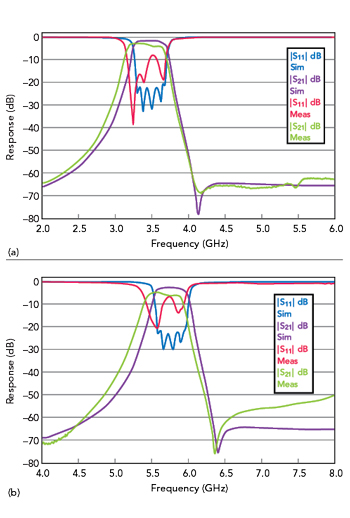
Figure 18 (a) 3.5 GHz measured and simulated results (simulation is in red). (b) 5.8 GHz measured and simulated results (simulation is in red).
Conclusion
For RF and microwave frequencies below 6 GHz, this lumped element approach to filter realization has significant advantages. For moderate to broad bandwidths, these techniques can produce useful results with an SMT approach, especially if the designer is aware of the impact of parasitics and filter topology have on design choices. At lower frequencies, the SMT filter is smaller than its distributed equivalent, has broad stopbands and is easier to tune, if necessary.
References
- Modelithics CLR Library, Modelithics, Inc., Web: www.modelithics.com.
- Cadence AWR Microwave Office, Cadence Design Systems, Inc., Web: www.cadence.com.
- EQR_OPT_MWO Optimization Software, DGS Associates, LLC., Web: www.dgsboulder.com.
- 4. Accu-P Capacitors, KYOCERA AVX, Web: www.kyocera-avx.com.
- J. K. Skwirzynski, “Design Theory and Data for Electrical Filters,” D. Van Nostrand Company LTD, 1965.
- Abside Networks, Inc. Acton, Mass., Web: www.abside-networks.com.
Appendix A
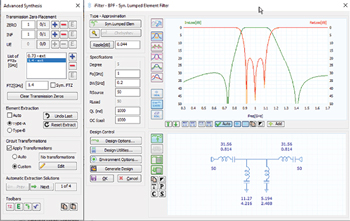
Figure 19 Cadence AWR iFilter display.
Starting with V18, the Cauer-Chebyshev elliptic filter can be synthesized using
Cadence AWR iFilter, with a representative display shown in Figure 19.
Enter the filter specifications in the Main Dialog: Fo = 1 GHz, BW = 0.2 GHz, Ripple = 0.044 dB.
In the Advanced Synthesis Dialog, Transmission Placement Group:
- Click Clear Transmission Zeros
- Click + on the first row to set ZERO=1
- Click + on the second row to set INF=1
- Click + next to the FTZ list and add a finite TZ (FTZ) at 0.73 GHz
- Click + next to the FTZ list and add a finite TZ (FTZ) at 1.4 GHz
In the Element Extraction group:
- Uncheck Auto
- Check Type-A
In the Circuit Transformations group:
- Uncheck Apply Transformations
Now do the element extraction:
- While 1.4 GHz is selected in the FTZ list, Click E next to the FTZ list
- While 0.73 GHz is selected in the FTZ list, Click E next to the FTZ list
- Click E next on the ZERO row
- Click E next on the INF row
*Observe the schematic in the Main Dialog.
INDser/SLCsht/CAPser/SLCsht is a specific quad topology that we will convert.
In the Circuit Transformations group:
- Check Apply Transformations
- Check Custom
- Click Edit
In the Circuit Transformations dialog:
- The top list is the existing macro
- Click Clear List if there is anything in that list
- Select ‘Replace 4-LC by 4-LC (Inv Geffe)’ from the available transformation list (fourth from the end)
- Click Add
- Select ‘Simplify Circuit’ from the list at the bottom left (fifth from the top)
- Click Add
- Click Close to close the dialog
*Now we have a macro that will replace all quad sections with an Inverse Geffe section (SLCser/SLCsht/SLCsht/SLCser). Geffe/InvGeffe are specific topologies arrived at by applying successive Norton transformations.
By checking/unchecking Apply Transformations, the effect of the macro can be seen.
Note the “Replace 4-LC by 4-LC (Inv Geffe)” transformation is new in V18 of Cadence AWR iFilter.
Note if an FTZ is selected and tuned by the mouse wheel, the whole extraction-transformation sequence will automatically update after every change.