

This article discusses critical antenna performance parameters commonly considered in low earth orbit (LEO) system operation and terminal design and reviews the regulations governing them.
LEO constellations consist of multiple satellites operating in a distribution of orbital planes. Each satellite transmits one or more beams, or footprints, in fixed or dynamic shapes and maintains coverage along the designated orbit. The coverage area of each satellite is determined by system parameters, including orbital altitude, target throughputs derived from link budgets and regulations like the International Telecommunications Union’s (ITU) power flux density (PFD) and equivalent power flux density (EPFD) limits.
A user terminal (UT) maintains its connectivity to the LEO system by tracking a designated moving satellite. Terminals must switch (hand over) links from a designated satellite to the next one when the terminal antenna reaches its limit of scanning range or when the satellite footprint moves away. Terminal antenna design and performance is, therefore, a critical parameter for system operation. A terminal’s complexity and cost also significantly impacts the viability of a network’s business model.
ANTENNA PERFORMANCE PARAMETERS
Effective Isotropic Radiated Power (EIRP)
EIRP measures a transmitter's performance by combining the transmitted power emitted with antenna gain.1 The EIRP of an antenna system is defined as:2
Where PT is the transmitter output power, GT is the gain of the transmitting antenna, and LC is signal attenuation in the feed between the transmitter and the antenna.
To achieve a target EIRP, designers can either enlarge the antenna aperture dimension (increase GT) or increase the transmitter output power (enhance PT). These two parameters, however, cause different concerns for the antenna system. A larger antenna aperture equates to higher gain (a more directed main beam) and a larger device form factor. Some mechanically steered flat-panel antennas require more powerful motors to drive the larger apertures; and, at higher frequencies pointing error and pointing loss can be significant. Transmitter pouwer level drives the cost of the power amplifier and the DC power consumption of a terminal. Higher power levels also generate waste heat in the antenna system and reduce G/T performance, which is sensitive to the ambient temperature of electronic components.
Gain to Noise Temperature Ratio (G/T)
G/T is a figure of merit that indicates a receiver’s performance, where G is the receive antenna gain, and T is the noise temperature of the system measured in Kelvin. From a system perspective, G/T dictates the antenna and RF front-end carrier-to-noise ratio, thus impacting the overall terminal throughput.
Two sources of system noise are the antenna noise temperature and the receiver noise temperature. Antenna noise temperature is due to background radiation in the antenna’s environment, i.e., the sky or the ground. Receiver noise temperature comes from components with dissipative losses, electronic noise and reflection losses that generate noise.1
To calculate system noise temperature at an antenna’s output, before any feed loss, the following equation can be used:3

where TA is the antenna noise temperature, TF is the feed operating temperature, TeRX is the effective input noise temperature of the receiver and LFRX is the receiver feed loss, which is inversely related to the gain at the receiver, i.e., GRX = 1/LFRX.
If the system noise temperature is calculated at the input to the receiver, after the antenna and any feed loss, replacing GRX with 1/LFRX, the system noise temperature can be calculated using the following equation:

It is imperative to ensure that the receiver reference stage at which G/T is calculated is clearly specified. In addition, in an array aperture where multiple radiating elements contribute to the gain and directivity, G/T comprises each individual element’s passive gain, each individual channel’s electronic gain, and the associated coherent noise combined through the network. The active electronic gain supporting each passive element effectively manages the noise caused by the passive transmission lines and combiners. This results in the following complex G/T calculation:4

where N is the number of channels, Ge is the element passive gain, η is aperture efficiency, Ti is the antenna sky temperature at the input, T0 is room temperature, Lf and Ld are the front-end and downstream losses respectively, Lk are the differential weightings of each channel, F is the noise figure of the low noise amplifier (LNA), and g is the electronic gain of the LNA. For antennas with power tapering or non-uniform elements, this formula must be extended to consider the summation of each individual channel’s characteristics.
Polarization and Cross Polarization
Polarization is a property of electromagnetic (EM) waves that specifies the geometric orientation of the electric field oscillations perpendicular to the direction of propagation. An EM wave is called unpolarized if the direction of the electric field fluctuates randomly in time.5 Most antennas are either linearly or circularly polarized.
Linearly polarized antennas are polarized in the horizontal or vertical direction. The electric field of a horizontally polarized antenna is parallel to the surface of the earth. Similarly, the electric field of a vertically polarized antenna is perpendicular to the surface of the earth.6
The electric field of a circularly polarized antenna radiates circularly once per wavelength. If the radiation pattern moves in a clockwise direction then the antenna is said to be right hand circularly polarized. Conversely, if the radiation pattern moves in a counterclockwise direction then the antenna is left hand circularly polarized. The polarization of a receiver and a transmitter must be matched for maximum signal integrity at the receiver. Even a slight mismatch in polarization can result in decreased signal strength.
The term co-polarization (Co-pol) refers to the desired polarization component of an antenna while cross polarization (X-pol) is the polarization component orthogonal to the desired polarization component. If an antenna is horizontally polarized, Co-pol is in the horizontal plane while X-pol is in the vertical plane. X-pol is usually unwanted noise.7
Radiation Patterns and Sidelobes
The graphical representation of an antenna’s radiation property, in 2D or 3D space, is its radiation pattern. 2D radiation patterns can be constructed by keeping a fixed azimuthal angle and varying the elevation angle, or by keeping a fixed elevation angle, and varying the azimuthal angle. These patterns are referred to as horizontal patterns and vertical patterns, respectively.8
The distinguishing characteristics of radiation patterns are their lobes. The main lobe is the angular region of maximum radiation, while the side lobes and minor lobes represent radiation in undesired directions. A null lobe represents a zone of zero radiation. Main lobe steering and null lobe steering are important techniques used to direct the beamforming pattern of an antenna.
Tapering
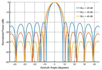
Figure 1 Normalized array factors of a 16-element uniform linear array with side lobe levels at – 20 dB, – 30 dB and – 40 dB.
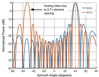
Figure 2 Normalized array factor of a 64-element uniform linear array with element spacings of 0.5 and 0.7 λ.
Tapering is the process of assigning different gains to the various elements within an antenna array, where the center elements are assigned the highest gains, and the outer elements are assigned lower gains. Sharper tapering, i.e. quickly reducing the element gain of elements farther from the center of the array, results in greater suppression of undesired side lobes. Compared to a similar-sized array with uniform gain across every element, however, a tapered array has reduced beam directivity and broader beamwidth.9
An example of tapering is shown in the array factor (radiation pattern) for a 16-element uniformly spaced linear array (ULA) of isotropic radiators at a center frequency of 19 GHz and progressively sharper tapers (see Figure 1). The yellow radiation pattern with sharpest tapering (sidelobe level (SLL) of -40 dB) has the broadest beamwidth while the blue curve with the least amount of tapering (SLL of -20 dB) has the narrowest beamwidth.
Grating Lobes
A replica antenna pattern caused by the incorrect spacing of radiating elements is defined as a grating lobe. In phased array antennas, the antenna elements spatially sample the incident wavefront. The Nyquist theorem can be extended to the spatial domain if we consider that two samples, or antenna elements per wavelength are required to avoid aliasing. If the element spacing is greater than λ/2, the resulting grating lobes are considered spatial aliasing.10