
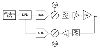
Figure 1 Architecture of a PA with DPD.
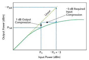
Figure 2 PA output vs. input power, where Pin drives the PA to 1 dB compression.
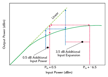
Figure 3 PA output vs. input power, showing Pin + 0.5 dB.
This article provides insight into the engineering of digital predistortion (DPD) systems for success, debunks some of the common misconceptions and gives real-world DPD performance examples.
In recent years advances in the performance of DPD for amplifier linearization have been largely driven by the cellular sector and the quest for higher power efficiency, spectral efficiency and data throughput with each successive generation of the standards. The complex modulations employed by standards such as 3G, 4G and 5G demand a level of transmission linearity significantly in excess of that offered by the power amplifier in isolation. This mandates linearization techniques to meet exacting out-of-band and in-band distortion levels as specified by the spectral emissions and modulation error requirements of the relevant standard.
DPD has particular relevance to 5G as the higher modulation bandwidths presented by many use cases that have the tendency to increase the level and complexity of non-linearity exhibited by a power amplifier (PA), the mechanisms for which are explored within this text. This puts a greater emphasis on ensuring that PAs are designed to maintain the extent of their non-linearities within the linearizer correction capabilities. Additionally, the very high data rates afforded by 5G consume significant power in transmission with respect to previous standards, notwithstanding the spectral efficiency of the modulation. Many wireless infrastructure sites have finite power supply networks that must still power the existing 2G/3G/4G infrastructure, to say nothing of the environmental implications of the power consumed. These factors place greater emphasis on a DPD’s ability to enhance 5G transmitter power efficiency and consequential savings in capital and operating expenses.
The latest generation DPD solutions trail-blazed by the cellular industry are now increasingly being deployed to other sectors including broadcast, satellite and private mobile radio as they in turn seek higher spectral efficiency through evolved, more sophisticated linear modulation.
DPD THEORY OF OPERATION
A simplified DPD system architecture is shown in Figure 1. The forward path comprises the wireless physical layer (PHY), DPD, digital-to-analog conversion, RF up-conversion and the target PA, while the feedback or observation path comprises RF down-conversion and analog-to-digital conversion.
In basic terms, DPD compensates for PA compression by expanding the input waveform. Figure 2 shows a nominal amplifier compression characteristic, which demonstrates that for this characteristic an input signal at level Pin is subject to 1 dB output compression (P1dB). Compensation of the compression characteristic requires 3 dB of input signal expansion, at which point the output power equates to that which would be provided by a linear characteristic (Pout(lin)).
Figure 3 illustrates the implications of now seeking an additional 0.5 dB of linear output power (Pout(lin) + 0.5). This new operating point requires an additional 3.5 dB of expansion for a total input signal expansion of 6.5 dB and the output power is again restored to that which would be provided by a linear characteristic. However, the drive level is now increased such that the PA is at the point of saturation (the PA characteristic has a near-zero or zero gradient) and no amount of further signal expansion will increase the output power. This illustrates an important concept in predistorter design, that the required input signal expansion generally increases exponentially with drive level and that operation at, or close to, PA saturation is undesirable. Saturated operation can be problematic for the predistorter adaptation algorithm and the high level of signal expansion consumes digital dynamic range, raising the associated noise floor.
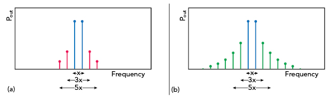
Figure 4 PA two-tone output spectrum without linearization (a) and corresponding input correction signal (b).
Perhaps the most common question to arise in predistorter design is how to determine correction (forward) path bandwidth. Figure 4a shows the two-tone unlinearized PA output spectrum with just third and fifth order intermodulation distortion products (IMD3 and IMD5) visible. Nonlinear theory of predistortion is outside the scope of this discussion, but it shows that full correction of an intermodulation product, in fact, requires a correction signal comprising an infinite series of odd-order products1 as illustrated in Figure 4b. Of course, an infinite correction bandwidth is not available in any practical system and a compromise is required. In reality, the ensemble of correction products above a certain order will have an insignificant performance benefit.
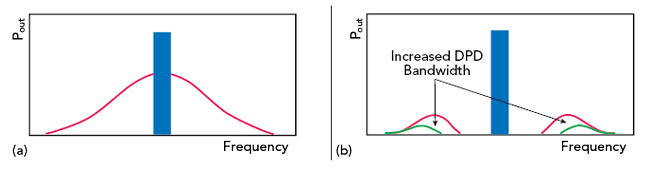
Figure 5 PA spectrum without linearization (a) and linearized PA output, showing improvement with larger correction bandwidth (b).
Figure 5a illustrates the unlinearized PA output for a broadband transmission. The effect of truncating the series of correction products within the PA input waveform is to introduce “bumps” of residual distortion within the output (see Figure 5b). The optimum correction bandwidth reduces the level of this residual distortion to the point where it falls within the specification plus appropriate margins.
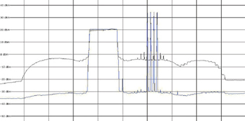
Figure 6 Output of a Doherty PA with 4G and multi-carrier 2G signal, with and without DPD linearization. Frequency range: 841.6 to 1001.6 MHz. Mean output power: 46 dBm.
Typically, the baseband correction bandwidth may be 4 to 5x the composite modulation bandwidth (i.e. at 5x it encompasses all fifth order predistortion products), though this figure of merit can vary significantly according to application and performance requirements. The transmitter’s digital and analog forward path must maintain this bandwidth to faithfully present the correction signal at the PA input. Therefore, for a 100 MHz modulation bandwidth the system may support a 400 to 500 MHz correction bandwidth from the baseband predistorter to the PA input, using the 4 to 5x guideline.
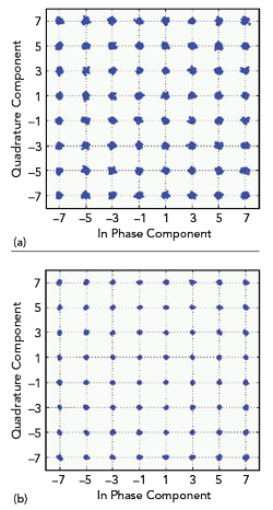
Figure 7 64-QAM constellation before linearization, MER = 33.1 dB (a) and linearized, MER = 39 dB (b).
While simulation has its place in determining the required correction bandwidth for a given scenario, the nonlinear hardware-in-the-loop nature of the problem means that the only reliable way to establish the bandwidth with certainty is by empirically evaluating the PA hardware within the DPD control loop. This approach provides a definitive answer as to what correction bandwidth achieves the desired spectral emission and modulation error levels. Fortunately, it is often possible to achieve this using off-the-shelf signal processing and radio transceiver evaluation cards without committing to the cost of prototype development.
Figure 6 illustrates the level of performance available from a latest generation digital predistorter. The mixed-mode signal (4G plus multi-carrier 2G) has a total instantaneous bandwidth of 40 MHz. It is illustrative of the current cost-driven push to share radio infrastructure and represents a challenging composite signal use case for any digital predistortion system. The Doherty amplifier has 46 dBm mean output power and the traces show performance with and without linearization enabled. For this scenario the level of third order intermodulation distortion is improved by up to 30 dB, from a highly nonlinear starting point. Of note is the DPD’s in-band equalization of the amplifier gain slope apparent on the 4G signal prior to linearization; this is one of the side benefits of DPD systems supporting this capability.