The radar systems that operate over broad expanses of land and sea surfaces, the fidelity of a simulated scenario is driven by how closely the scenario represents these surfaces. For some radar systems, the returns from these surfaces are unwanted and are referred to as clutter. Radar system engineers and radar signal-processing analysts are focused on removing the effects of this clutter to detect targets.

This next Code & Waves blog will discuss sea surface modeling concepts to generate plan position indicator (PPI) radar images for a maritime scenario. These images will then be used to train and evaluate a convolutional neural network (CNN) to mitigate clutter returns.

Simulate a Maritime Radar PPI

The presence of sea clutter in maritime radar applications is sometimes not desired and interferes with a radar’s ability to detect targets and estimate their physical characteristics. To improve detection of targets of interest and assess system performance, it’s important to understand the nature of returns from sea surfaces.

Let’s start by considering a radar scenario that consists of an X-band radar system operating at 10 GHz. This radar has a horizontally polarized, rotating uniform rectangular array (URA) mounted in a fixed position of 24 meters above a moving sea surface. The radar has an azimuth beamwidth of 1 degree and 10-meter range resolution. For our first example, we will model returns from a medium-sized container ship, moving at a rate of 8 m/s. This target is modeled using a set of discrete scatterers along the surface of a cuboid of size 120 m long x 18 m wide x 22 m high with a radar cross section (RCS) of 10 m². The spacing of the scatterers along the cuboid is determined by the azimuth and range resolution of the radar.

Next, we will consider a moving sea surface representative of a sea state 3. The reflectivity of this sea surface will be based on the NRL model, one of the 9 built-in models in Radar Toolbox appropriate for sea surfaces. The wave elevation spectrum and angular distribution will be based on the Elfouhaily model. The Elfouhaily model will dictate the movement of the sea’s waves. The clutter from this sea surface will be simulated within the 3 dB width of the radar’s main beam. Shadowing, which occurs when a surface return is occluded due to surrounding surface features, will be considered. Figure 1 shows the full radar scenario.

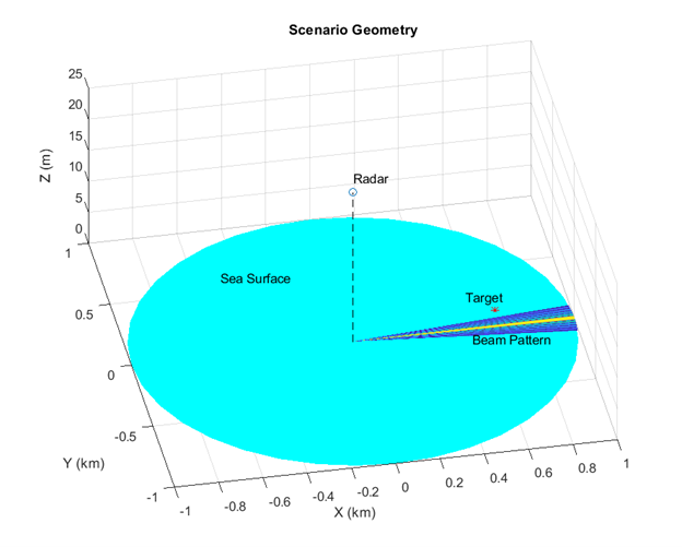
Figure 1: Maritime scenario with a rotating radar system. The radar, empty blue circle in the center of the image, is mounted above the sea surface at 24 m. The target position is shown as a red asterisk. The 3 dB width of the radar main beam is plotted on the sea surface, which is denoted by the cyan disk. ©2024 The MathWorks, Inc.

Now that we have our maritime scenario, we will generate IQ signals and match filter the returns. Each frame of the simulation generates a range profile for one azimuth pointing direction. A PPI image consists of a set of range profiles arranged in radial lines to form a circular image of a scene in Cartesian space. In Figure 2, the scan starts at 0 degrees azimuth and proceeds to cover an area of 45 degrees, which is enough to see the target in the specified geometry.

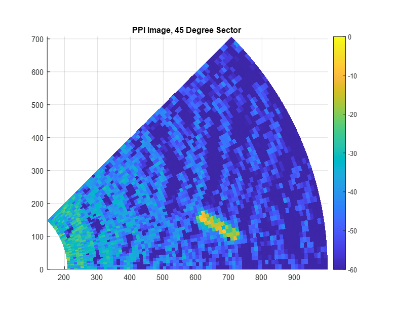
Figure 2: Maritime PPI image covering a sector from 0 degrees to 45 degrees. The simulated medium-sized container ship is visible as the yellow, rectangular section. ©2024 The MathWorks, Inc.

By continually adding range profiles to the PPI image, a full rotation can be completed and visualized as in Figure 3.

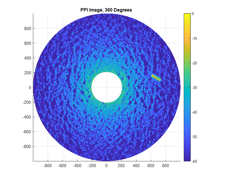
Figure 3: Maritime PPI image covering a full 360 degrees. ©2024 The MathWorks, Inc.

Mitigating Sea Clutter Using Deep Learning

Mitigating sea clutter is even more challenging than land clutter due to the motion of the waves. Many conventional clutter mitigation techniques are tailored to stationary ground clutter, so using these techniques on dynamic sea clutter sometimes produces unsatisfactory results. As such, we can consider alternative means such as using deep learning to remove clutter returns and improve target detectability.

Let’s consider a dataset containing 84 pairs of simulated PPI images based on the scenario previously discussed. Each pair consists of an image that includes target and sea clutter returns and a desired response image that contains only targets as depicted in Figure 4. We will use about 95% of the data for training and validation of the network, with the other data being used for testing the network.

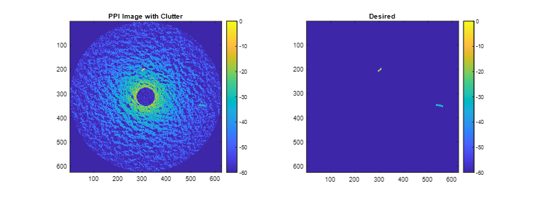
Figure 4: Image on the left is a maritime PPI image that includes sea clutter and extended target returns. The image on the left is the desired image that contains only targets. These two images are one of the 84 image pairs that are used to train and validate the CNN network. ©2024 The MathWorks, Inc.

Each image contains two nonoverlapping extended targets with one representing a small container ship and the other representing a large container ship. We will model these targets in the same way as before by approximating the targets as a set of point scatterers on the surface of a cuboid. The small target is 120 x 18 x 22 m, and the larger target is 200 x 32 x 58 m.

To ensure the network is applicable to a wide range of scenario geometries and sea states, we will vary target position, heading, and speeds. Similarly, we will randomize the sea surface conditions with wind speeds ranging from 7 to 17 m/s and wind directions between 0 and 180 degrees.

A network is defined by a sequence of layers, including input and output layers. Our CNN network will consist of 11 layers in total. The proposed network ingests the images and processes them through a cascade of 3 sets of 2-D convolutional layers, normalizations, and a non-linear activation function. Each convolutional layer spatially filters the images. The normalization layers bias and scale the images to enhance numerical robustness and improve the training. The activation layer in this case is a leaky rectified linear unit (leaky ReLU). A leaky ReLU improves learning in comparison to a standard ReLU activation function in that it prevents “dead neurons”, a situation that occurs when values become negative. The final output layer of this network is a regression layer, which implements a simple mean-squared-error (MSE) loss function. Overall, the layers result in a network with 287 learnable parameters. An overview of the neural network architecture is depicted in Figure 5.

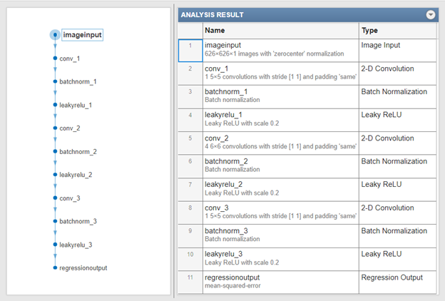
Figure 5: Image on the left shows a flow diagram of the CNN network. The table on the right has additional information about the layer type and configuration. ©2024 The MathWorks, Inc.

The network is able to completely remove the clutter below a certain threshold of returned power while retaining the target signals with only a small dilation effect due to the size of the convolution filters used. The remaining high-power clutter near the center of the image could be removed by adding a spatially aware layer such as a fully connected layer. Another way to improve performance is to perform pre-processing of the original images to remove the range-dependent losses.

In this example, you saw how to generate clutter and target returns with a rotating radar in a maritime environment. You saw how to use a spectral model to get realistic sea surface and how to emulate an extended target with a set of point targets. The IQ data was converted from polar format to Cartesian and plotted to create a simple PPI image. A series of these PPI images were then used to train and evaluate a cascaded CNN network to remove sea clutter, while retaining target returns.

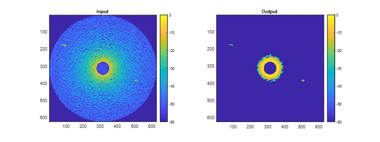
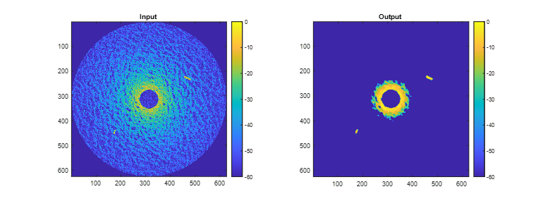
Figure 6: Images on the left are the maritime PPI that include sea clutter and extended target returns. The images on the right are the outputs of the CNN network. As can be seen, the neural network is able to remove the clutter to a great extent at the expense of a dilation effect on the targets. There is residual clutter power that is not mitigated, which could potentially be removed by adding fully connected layers to the network or performing pre-processing on the images prior to application of the network. ©2024 The MathWorks, Inc.

To learn more about the topics covered in this Code & Waves blog and explore your own designs, see the examples below or email abhishet@mathworks.com for more information.