Measurement Considerations

Measuring pulsed radar signals requires a peak power sensor. For fast pulses, the rise time of the power sensor is important. The Boonton RTP5006 has a rise time of ≤ 3 ns. This means that a pulse rising edge of 5 ns can be comfortably measured. The rise time display of a representative pulse is shown in Figure S-1.

Fast real-time and equivalent-time sampling provide fine resolution on narrow pulses. The RTP5000 real-time peak power sensors, with 100 MSa/s real-time and 10 GSa/s equivalent-time sampling, can make measurements on 10 nsec pulses with 100 psec resolution.

When measuring amplifier droop, automated measurements become important. Droop is one of the 16 automated pulse measurements available from the RTP5000 family. Figure S-2 shows the effects of droop on a reference signal.

RTP5000 power sensors may be used with a PC running the Boonton Power Analyzer Software or with the PMX40 power meter for a benchtop instrument experience. Either way, they provide an ideal tool to characterize radar and EW signals.

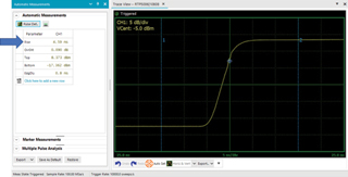
Figure S-1 Pulse rising edge with automated 10/90% rise time measurement shown by the blue arrow.

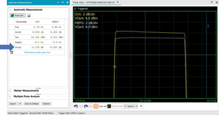
Figure S-2 Comparison of live trace with memory to see the effect of signal changes on droop.

RESULTS OF PRACTICAL IMPLEMENTATION

Figure 7 shows the measurement of the 40 kW SSPA output with the Boonton power sensor before applying the correction algorithm. This result was captured by the Boonton Power Analyzer Software. For a 500 μsec pulse width, the peak with overshoot measures 76.053 dBm. The end of the pulse top is measured at 74.36 dBm. The Boonton software captures the pulse envelope, which can be exported to a CSV table. From that table, the overshoot can be determined to settle around 75.2 dBm. The uncorrected pulse is then described as having an overshoot of approximately 0.9 dB (76.053 − 75.2 dBm) with a droop of approximately 0.8 dB (75.2 − 74.36 dBm).

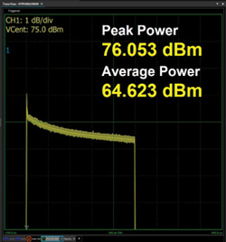
Figure 7 Uncorrected 40 kW pulse.

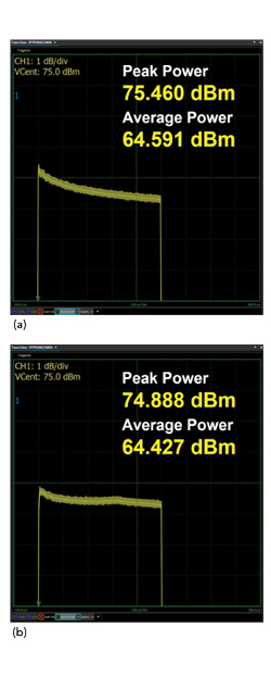
Figure 8 Response with overshoot correction applied (a). Response with slope droop correction applied (b).

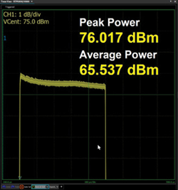
Figure 9 Response of the optimized result.

Figure 8a shows the effect of the overshoot correction stage, which decreases the overshoot by approximately 0.6 dB from the uncorrected pulse. Figure 8b shows the effect of the droop correction stage, which decreases the overshoot again by nearly 0.6 dB. While these stages decrease the amplitude of the overshoot at the front edge of the pulse, the trailing edge of the pulse remains unchanged. The effect reduces the overall energy of the pulse, a poor tradeoff for the benefit of flattening the pulse. Once the pulse is flattened, however, the gain of the system can be increased since the reduced overshoot will no longer activate the amplifier peak limiter. This is shown in Figure 9.

For the final result of Figure 9, the maximum peak power was adjusted by increasing the system gain. This results in a system gain higher than that of the uncorrected pulse example. For simplicity of illustrating the method, the gain adjustment has been described as the last step. In actual implementation, the correction factors are established ahead of time and stored, so setting the system to the optimized maximum gain is the first step. Next, the pulse rises and the overshoot is corrected with a final step of correcting the droop of the pulse.

SUMMARY

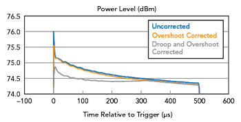
Figure 10 Impact of overshoot and droop correction.

The power output measured over the duration of the 500 μsec pulse is shown in Figure 10. This output demonstrates a flatter response with less overshoot that results from applying both droop and overshoot correction. In addition to providing more uniform power throughout the pulse, the amplifier can also generate higher average power. This is a result of higher system gain without fear of the overshoot activating the limiter and a pulse with less droop.

CONCLUSION

Using these techniques increased the average pulse power by 0.9 dB, which is close to the amount of pulse correction. This is as expected since the maximum transmitter output can be increased by the amount that the pulse variation is reduced. The result represents more than a 20 percent increase in average power, which also improves SWaP, cost and MTBF. The transmitter power density improves by 20 percent. The MTBF and cost improve since the component count in the RF chain would have been higher and the transmitter would have operated at a higher temperature to produce the 20 percent output power increase that would have been required without the pulse correction. In addition, the radar performance improves as roughly 1 dB of increased transmit power extends the range of the radar by 6 percent.