
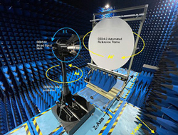
Figure 2 Image reflection setup.
Equation 10 represents the system magnitude and phase. If it is assumed that the AUT is lossless, then S11 = S22 where S11 is relative to a 50 ohm source and S22 relative to a 377 ohm load. To establish an [S] matrix for the AUT, the phase center must be known relative to the connector. The AUT shown in Figure 2 uses a lens that also serves to maintain a somewhat constant phase center location. This is measured using a least squares convergence algorithm for phase center offset (PCO) determination. The AUT measured |S21| data is given phase, based on the PCO value. Equation (7) is replaced with

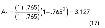
To calculate S22 it is necessary to transform S11 from 50 ohms to 377 ohms. These types of transformations were originally derived by G. Bodway5 as

where

and

and
With the previous assumptions the antenna scattering matrix may be written as

VERIFICATION MEASUREMENTS
Verification is performed on a very broadband (500 MHz to 30 GHz) reference horn. The image reflection setup uses a Diamond Engineering DE0540 horn antenna and an aluminum sheet at distance R (see Figure 2). Antenna gain and phase is determined from S11 measurement. The phase center is determined to be 228.6 mm.
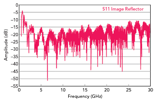
Figure 3 Measured |S11| of the DE0540 horn at boresight and radiating into a conductive sheet.
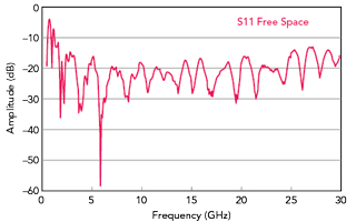
Figure 4 Measured |S11| of the DE0540 horn with absorber between the horn and conductive sheet.
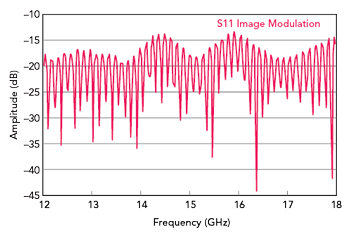
Figure 5 Modulation of the AUT image reflection.
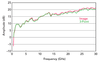
Figure 6 Measured image (red) and 3-point (green) gain.
The gain of the AUT ranges from 3 to 23 dB. The conductive surface is set perpendicular to the AUT using a laser and an optically flat mirror. The sequence is to first measure the AUT S11 magnitude and phase directly pointed into the surface. Then the measurement is repeated after the absorber is placed between the surface and the horn, nearer the horn. Figures 3 and 4 show the measurement results.
A magnified view of Figure 3 (see Figure 5) reveals the modulation of the AUT match profile. Since the reflection repeats every half wavelength, the distance between the source and mirror is:

The reflection ripple in Figure 5 is easily filtered using a moving average. The number of points should be large enough to include at least three points in a single reflection cycle. The number of measurement points over the bandwidth generates the following measurement frequency steps:

where BW is the measurement bandwidth and n is the number of measurement points.
From Figure 5, the path generates a reflection ripple of 133.3 MHz. If the measurement spanned 1 to 30 GHz, then the minimum number of measurement points would be  or 654. The measurements in this work use 2001 points.
Applying Equation (13) to Figures 3 and 4 and performing the moving average yields Figure 6.
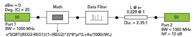
Figure 7 Schematic construct used to calculate S21 and S22.
S-Parameter Determination
Measurement data is processed through a schematic construct (see Figure 7) enabling Equation (18) to be calculated. Figure 8 shows the complex S21 polar plot. S22 (see Figure 9) is calculated from Figure 7 by changing the output impedance from 50 to 377 ohms. Using the calculated results from Figures 8 and 9 and the measured S11 completes the [S] matrix for the AUT.
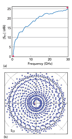
Figure 8 |S21| (a) and linear polar S21 (b) responses.
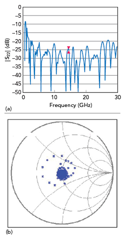
Figure 9 |S22| (a) and linear polar S22 (b) responses looking into free space (377 Ω).