In this blog post, we continue our investigation into a VRM’s Power Supply Ripple Rejection (PSRR) performance. In earlier posts, we reviewed PSRR concepts by running a couple of simulations and now we power up a real VRM in the lab.
Our DUT (Device under Test) is the VRTS1.5 ‘Voltage Regulator Test Standard’ from Picotest (thanks to Mr. Steve Sandler for the board).
By using the Bode 100 Vector Network Analyzer (VNA) from Omicron Lab, together with the J2121A High Power Line Injector (though it doesn’t need to be ‘high current’ - this is what I had available in my lab), we get this PSRR plot (Figure 1).

My lab setup obtaining this curve is shown in Figure 2. In this setup, everything is straightforward except for one point: I’m using four series load resistors of 50 Ω each, total 200 Ω, into the 50 Ω terminated input ‘port 1’ of the Bode 100 unit, to form ×1/5 attenuation. This avoids too high current loading on the VRTS1.5 DUT.

Some quick observations:
- The unit maintains high PSRR across a wide bandwidth, with the benefit of its voltage follower/buffer structure.
In other words, ‘N-type’ linear regulators/LDOs are generally better for PSRR compared with ‘P-types’. - In the low frequency region, below 10Hz, this declining curve is an artificial result from my measurement setup. I confirmed that my perturbation signal is not fully delivered to the DUT in this frequency region and my Bode 100 unit struggled to pick up a meaningful signal from the noise floor.
- One advantage of this VRTS1.5 DUT board is that there is no bypass capacitor at its power input. So, this simple setup with ten to fifteen minutes of effort brings me a result.
Any PSRR measurement of a switch mode power supply (SMPS) is not this easy, as we must have a certain minimum amount of input bypass capacitance.
This RF signal integrity to power integrity series focuses on ‘integrity’ studies and I leave further discussions on how to measure PSRR for another time. From this PSRR result, here is my first message in this post:
We electronics engineers handle many parameters in the form of a ratio, such as a unit of gain in dB, or efficiency in percentage. These parameters are generally a ratio of ‘something input’ to ‘something output’. For example:
Efficiency, power or energy [%] | η = 100 x (Output power [W] or energy [J])/(Input power [W] or energy [J]) |
PSRR [dB] | 20 log (Input voltage/Output voltage) |
(Amplifier) Gain [dB] | A = 20 log (Output signal voltage/Input signal voltage) |
As our electronics components evolve day by day to higher and higher performance levels, by chasing these parameter specification numbers, we tend to forget what was/is behind ‘input and output’ quantities. It’s useful to get back to basics from time to time.
Now, in my Excel program, I just tweaked the same VRTS1.5 PSRR curve (Figure 3). It shows exactly the same data but uses a different way of mathematically expressing the Y-axis, absolute values rather than dB.
In this graph, we can see how big an output ripple voltage (Y-axis) we have at our frequency of concern (X-axis) from an input supply of 100mV ripple amplitude. As you can see, it’s the same shape as the original PSRR curve, but just horizontally mirrored.

I hope this way of showing PSRR data brings a clearer idea of what your VRM does for you in terms of ripple rejection as a filter.
In power electronics designs handling 3.3 or 5 V power rails, a power supply of 100 mV ripple would be considered fairly ‘dirty’. For example, if you have 2 power rails of 3.0 and 3.3 V in your system and if you were dealing with 100 mV peak-to-peak ripple on both rails, you don’t have much clearance/margin in between, resulting in not having much value in having 2 rails when only one at 3.15 V might be enough.
This graph might suggest that such a ‘dirty’ power rail will be cleaned up to a level below 100 μV to 1 mV. From this you might be thinking: ‘Yes, that’s why I need an LDO to clean up my power supply’.
Here is my second message in this post:
When taking measurement data, we always double- or triple-check the result using alternative ways/methods. For example, when taking data in the time domain, it can be validated by frequency-domain data and vice versa.
So, I connected an arbitrary function generator (AFG) and oscilloscope probes to the positions I used for my VNA. Then, I injected 100 mV input ripple to see if I can get the same ‘ripple in, ripple out’ results as shown in the previous curve.
The following six waveforms (Figure 4 to 9), were recorded at 10 Hz, 100 Hz, 1 kHz, 10 kHz, 100 kHz and 1 MHz as shown in the captions.
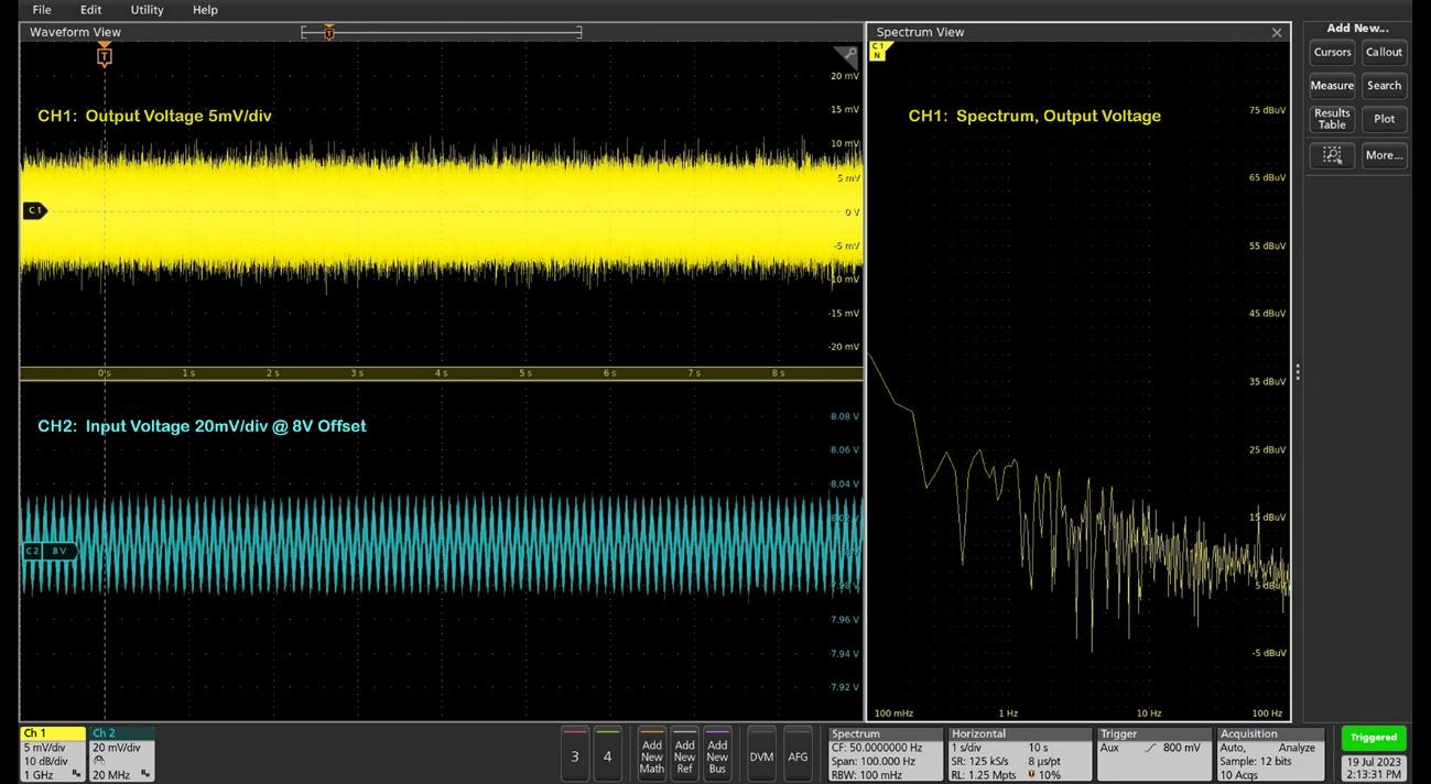
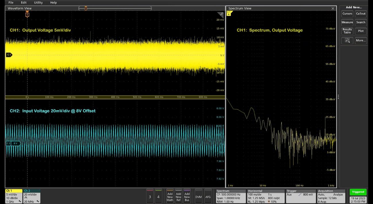

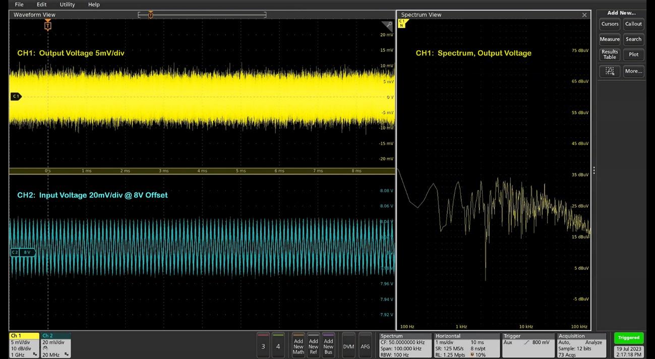
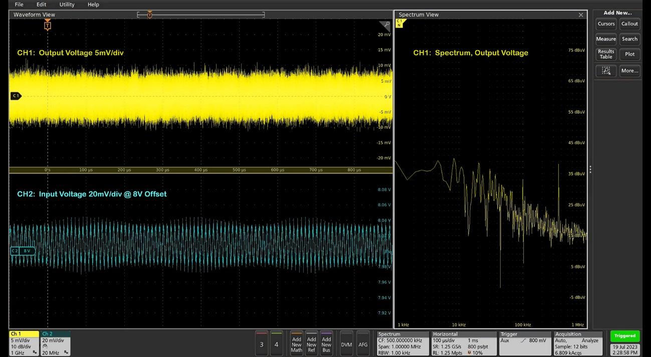
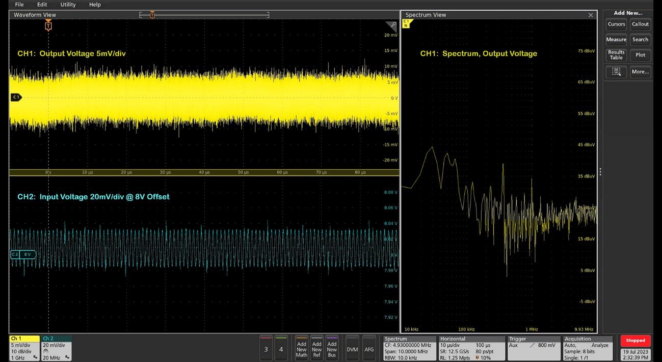
And from these 6 waveforms, you see my 2nd message clearly regarding the myth of PSRR. In the real world, most VRMs self-generate bands of output noise at the scale of millivolts. You can only find this when you run the alternative measurement staying out of the frequency domain.
In the frequency-domain PSRR measurements, your VNA knows exactly the frequency of the ripple input into the DUT and it picks up the output ripple by a synchronization circuit. That’s why it can generate nice, clean PSRR curves.
As you can imagine, the VNA is picking up the output ripple signal from the deep bottom of the noise floor.
I’m not totally denying the value of a VRM’s PSRR performance here. If you know your pinpoint frequency of concern, a VRM of high PSRR at your target frequency will do a good job. For example, in a system where you know there is a noise source that you cannot remove, such as a big motor spinning and injecting noise spikes back into the power line at a known repetition rate. Perhaps the motor noise showed up as a result of data logging.
But if your concern is general noise, for example as described in this article, you may want to find a ‘low noise’ VRM instead of one with ‘high PSRR’. In my experience, in many, many cases, engineers need ‘low noise’ VRMs more than ‘high PSRR’.
The previous six waveforms are extreme examples, showing measurements down near your noise floor. We can also make following key observations.
- My bench setup has a noise source coupled through the ground line at 350 kHz which can be found in waveforms at 100 kHz and 1 MHz. At 100 kHz, we have a beat frequency between the main 100 kHz ripple input and this 350 kHz ground noise.
- The VRM self-generated noise is strong at low frequency. At 100 kHz to 1 MHz, the spectrum of output ‘noise + ripple’ can show the spurs we are looking for. Still, we can see this spur is not the dominant one and we can’t see it in the time-domain waveforms.
- I controlled the output signal from the AFG at 100 mV, and the actual delivered input ripple at the DUT board is slightly less through the J2121A injector. The VNA compares actual probed signal at the DUT board and it makes no significant impact on the PSRR measurements.
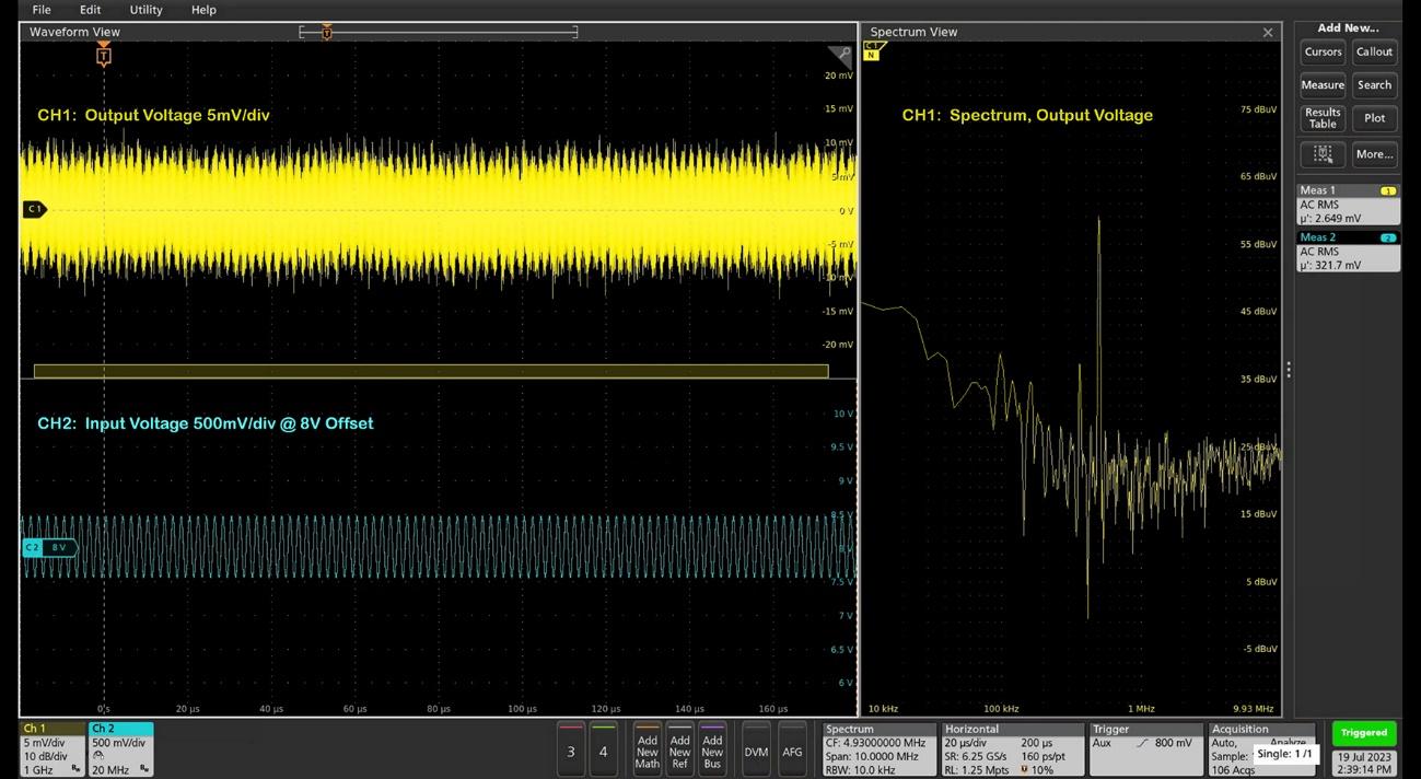
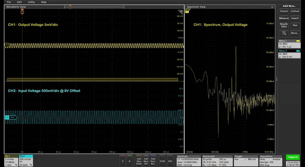
- To validate this setup by comparing time domain and frequency domain results, I have the following additional waveforms (Figures 10 and 11). Getting visible output ripple in the time-domain, we need 1 V input ripple for this high-PSRR DUT. Furthermore, we need to average out the waveform to eliminate random noise. With the final waveform, we can calculate 50.6 dB of PSRR at 500 kHz which matches well with the original PSRR curve of this post.
PSRR@500 kHz = 50.6 dB = 20 × log (322.0 mV/951.7 uV)