
Radar has evolved from a complex, high-end military technology into a relatively simple, low-end solution penetrating industrial and consumer market segments. This rapid evolution has been driven by two main factors: Advancements in silicon and packaging technology are leading to miniaturization, and growth of computing power is enabling the use of machine learning algorithms to tap the full potential of raw radar signals. Radar facilitates localization of targets in 3D space and can be further used for vital sensing or classification, providing a 4D view that enables several industrial and consumer applications. The use and applications of radar technology have grown multi-fold in recent years. Apart from military and defense applications, radars increase safety and facilitate driving in medium- to premium-priced cars, for example. For many industrial and consumer applications, the wide adoption of short-range radar sensors follows reliable system performance at low-power and low-cost. In this article, we explain how radar technology can be used in consumer electronics and industrial applications, bringing benefits to our daily lives.
Radar supports existing applications while providing features that enable completely new use cases. Radar 3D localization in home and industrial applications provides range and angle, both in azimuth and elevation. Radar can also sense velocity for position mapping and tracking. Specialized radars can detect human cardiopulmonary motion, providing a promising approach to overcoming problems of false triggering and dead spots in conventional sensors for occupancy sensing. Radar technology produces a unique signature for any object or material. This feature can be used in systems to recognize different types of liquids-water vs. milk-or materials-silk vs. cotton.
Low-cost sensor solutions are enabling radar’s use for industrial testing and automation. They are robust in harsh environments, such as poor lighting, fog or pollution. Additionally, they can be aesthetically concealed without affecting performance, making them suitable for many consumer applications. Radar has been demonstrated to be a powerful sensor for short-range localization and vital sign tracking within consumer electronics, medical care, surveillance, driver assistance and industrial applications.1-5
ENABLING TECHNOLOGIES
A radar system consists of two parts: First, the radar hardware, including the RF transceiver, waveform generator, receiver unit, antenna and system packaging. Second, the signal processing, which parses the radar return echo to extract meaningful target information.
Since the invention of integrated circuits, the operating frequency of transistors has steadily increased, enabling the realization of circuit blocks that operate at frequencies up to 1 THz.6 Transistors are also shrinking in size, with more advanced technology nodes enabling further integration.7 Figure 1 highlights the evolution of radar technology used in automotive applications. SiGe bipolar technology has been the preferred silicon technology for automotive and industrial mmWave radar for the past several years, as its performance, cost and integration fit superbly with application requirements.8-9 State-of-the-art SiGe technology has reached operating frequencies beyond 300 GHz. For example, Bock et al.10 describe front-end BiCMOS technology with an Ft of 250 GHz and an Fmax of 370 GHz for the SiGe transistors. Their technology also has 130 nm CMOS, which can be used for radar building blocks, such as phase-locked loops and digital signal processing. RF CMOS technology has also been shown to be a candidate for mmWave radar.11 Although RF performance is not as good as SiGe, CMOS offers greater digital integration, attractive for increased signal processing on the radar chip.
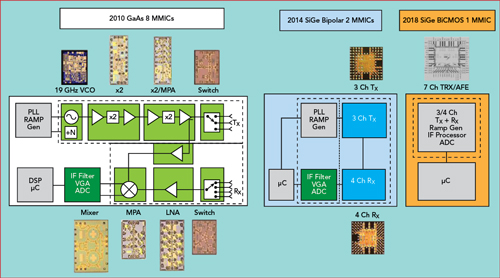
Figure 1 77 GHz radar transceiver technology and integration trend.
Higher operating frequencies and advanced packaging technologies have enabled the integration of antennas into the package and, in some cases, on the silicon die. Antenna integration is essential for reducing radar design complexity and for reducing overall system cost, allowing penetration into industrial and consumer markets. Antenna configurations have been integrated into packaging for different fields of view to cover various system requirements.12 Operation beyond 100 GHz allows the integration of the antenna on silicon,13 further reducing radar size and cost.
RADAR TYPES
Small short-range radars can typically be categorized as CW, modulated CW and impulse ultra-wideband (UWB).
CW Radar
CW radars transmit and receive continuously, while impulse radars transmit short pulses while the receiver is not operating and receive in the quiet period between transmit pulses. CW radars require separate transmit and receive antennas with good isolation. The major advantage of CW radars is that signal processing at the receiver is at low frequencies, reducing the sampling rate requirement, which simplifies processing circuitry.
CW radar transmits an unmodulated continuous frequency tone. The received echo is processed to estimate a target’s radial velocity by evaluating the change in phase with respect to time of the received signal relative to the transmitted signal. This Doppler frequency shift is from the transmitted signal reflected from a moving target. The disadvantage is range information cannot be obtained from a pure CW signal; it can only be obtained through either pulse-Doppler operation or transmitting two distinct frequency tones, known as frequency shift keying.
Modulated CW Radar
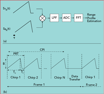
Figure 2 De-ramping the FMCW signal (a) and radar frame structure (b).
Several patterns are used to frequency modulate the transmit signal. A popular waveform is sawtooth frequency modulation, where the frequency is linearly increased over time (up-chirp) or decreased over time (down-chirp). This is called frequency modulated CW (FMCW). At the receiver, the matched filtering operation requires mixing the received chirp with the transmit signal, called “de-ramping” or “de-chirping” (see Figure 2a). STx(t) and SRx(t) refer to the transmit and the received chirp respectively. The round trip propagation delay

is translated to an intermediate frequency after mixing in the receiver. Spectral analysis along the chirp provides range estimates of targets in the radar’s field of view. The swept bandwidth, B, determines the range resolution, δR = c/(2B). The maximum unambiguous range Rmax = NsδR, where Ns is the number of transmit frequency steps. The analog-to-digital converter (ADC) output along a single chirp is referred to as “fast time.”
Figure 2b shows the frame structure of the FMCW radar. The chirp duration Tc determines the maximum detectable unambiguous Doppler, fdmax = 1/(2Tc). The time duration between two chirps is referred to as the pulse repetition time (PRT) and is given as PRT = Tc + Ti. The velocity content of a target within a range bin causes a phase change across multiple chirps within the target’s range bin. The spectral estimation across chirps provides the velocity information. The collection of consecutive chirps used for coherent integration is referred to as the “frame” or “dwell” and represents how often target parameters are estimated or updated. The coherent processing interval (CPI), the time duration of a frame, determines the Doppler resolution δfd = 1/(2CPI). The time samples along the chirps within the CPI are referred to as “slow time.” Two critical aspects that determine the performance of a sawtooth frequency modulated radar system are the ramp linearity and the transmit-to-receive (TX-RX) leakage. Any deviation from a linear ramp results in range estimation errors and the TX-RX leakage limits the radar’s maximum detection range.
Impulse UWB Radar
Impulse radar transmits short pulses and determines distance by measuring the time delay between the transmitted and returned signal. Impulse radar transmits ultra-wideband, short pulse waveforms and is a non-coherent system. The time difference between pulse transmission and reception determines the range of the target and the peak of the spectrum determines the Doppler velocity. The pulse width determines the range resolution and the Doppler resolution is typically poor in such systems; however, they do not suffer from TX-RX leakage, since the transmitter and the receiver do not operate at the same time.
This article introduces the concept of 4D sensing using FMCW radar. However, several aspects are applicable to impulse UWB radar.
3D POSITION LOCALIZATION
To estimate a target in 3D space, a MIMO configuration of at least NTx = 2 transmit elements and NRx= 2 receive elements in an L-shaped linear array with appropriate spacing is required. This results in a virtual 2 × 2 rectangular array sufficient for estimating a target’s elevation and azimuth coordinates.
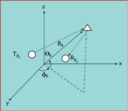
Figure 3 3D position of the target.
As shown in Figure 3, the 3D coordinates in space of the TX element are denoted as  = 1...NTX and for the RX element as
  = 1...NRX. Assuming far-field conditions, signal propagation from the TX element
  to a point scatterer p and the reflection from p to the RX element
  can be approximated as 2Rk + dmn, where Rk is the base distance of the kth scatterer to the center of the virtual linear array and dmn refers to the relative position of the virtual element to the center of the array. The radar views the space in polar coordinates, thus the 3D cartesian position of the kth target can be represented as

and the directional unit vector is represented as

where θk and φk are the elevation and azimuth angles, respectively, of the target with respect to the center of the virtual array. The transmit steering vector can be written as

while the receiving steering vector is

where λ is the wavelength of the transmit signal. The received baseband signal from the kth target scatterer can be expressed as

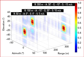
Figure 4 Estimated 3D position of three targets with different ranges and elevation and azimuth angles.
where ρk represents the composite amplitude contribution due to propagation path loss, antenna gains and receiver gains.  and
and  are the transmitted signal from NTX transmit antennas and the received signal at NRX receive antennas, respectively. After having estimated the range Rk of the kth target through spectral analysis along fast time, the angular coordinates of the target-namely azimuth angle θk and elevation angle φk-can be estimated through monopulse, Capon or FFT beamforming algorithms. Figure 4 shows the 3D localization of three targets with different positions (range, azimuth, elevation) in the radar’s field of view.
THE FOURTH DIMENSION
Vitals and Occupancy Sensing
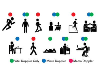
The breathing motion of human beings and heart motion from hearts beating have unique signatures that are picked up by radar as position and Doppler information.
A vibrating point scatterer target at base distance Rk from the center of the radar array induces a target response along slow time ts, which can be expressed as

where fv represents the vibrating frequency,  represents the maximum amplitude of the ith vibrating target source and I represents the number of vibrating sources. A quasi-stationary human at a fixed distance from the radar sensor can be modeled as the superposition of two vibrating sources: one from the respiratory motion, the other from heart motion. The human resting respiratory rate is around 12 to 20 beats per minute ( fv(1)= fr = 0.2 − 0.4 Hz), with a maximum displacement for chest wall motion = 7.5 mm. The heart rate can be from 50 to 200 beats per minute (f(2)v = fh = 0.8 − 3.3 Hz), with a maximum displacement α(2)v = 0.25 mm. After lowpass filtering, the received signal can be expressed as

Here, we expand the time index t as a combination of fast time, tf, and slow time, ts. The round trip propagation delay
