
Return Loss and Insertion Loss
Return loss is the ratio of the power level of the reflected signal to the power level of the input signal expressed in decibels (dB), i.e.,
RL (dB) = 10 log10 Pi/Pr (2)
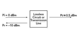
Figure 2 Return loss and insertion loss in a lossless circuit or transmission line.
In Figure 2, a 0-dBm signal, Pi, is applied to the transmission line. The power reflected, Pr, is shown as −10 dBm and the return loss is 10 dB. The higher the value, the better the match, that is, for a perfect match, the return loss, ideally, is ∞, but a return loss of 35 to 45 dB, is usually considered a good match. Similarly, for an open circuit or a short circuit, the incident power is reflected back. The return loss for these cases is 0 dB.
Insertion loss is the ratio of the power level of the transmitted signal to the power level of the input signal expressed in decibels (dB), i.e.,
IL (dB) = 10 log10 Pi/Pt (3)
Pi = Pt + Pr ; Pt/Pi + Pr/Pi = 1
Referring to Figure 2, Pr of -10 dBm means that 10 percent of the incident power is reflected. If the circuit or transmission line is lossless, 90 percent of the incident power is transmitted. The insertion loss is therefore approximately 0.5 dB, resulting in a transmitted power of -0.5 dBm. If there were internal losses, the insertion loss would be greater.
S-parameters
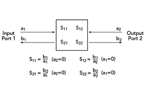
Figure 3 S-parameter representation of a two port microwave circuit.
Using S-parameters, a circuit’s RF performance can be completely characterized without the need to know its internal composition. For these purposes, the circuit is commonly referred to as a “black box.” Internal components can be active (i.e., amplifiers) or passive. The only stipulations are that the S-parameters are determined for all frequencies and conditions (e.g., temperature, amplifier bias) of interest and that the circuit be linear (i.e, its output is directly proportional to its input). Figure 3 is a representation of a simple microwave circuit with one input and one output (called ports). Each port has an incident signal (a) and a reflected signal (b). By knowing the S-parameters (i.e., S11, S21, S12, S22) of this circuit, one can determine its effect on any system in which it is installed.
S-parameters are determined by measurement under controlled conditions. Using a special piece of test equipment called a network analyzer, a signal (a1) is input into Port 1 with Port 2 terminated in a system with a controlled impedance (typically 50 ohms). The analyzer simultaneously measures and records a1, b1 and b2 (a2 = 0). The process is then reversed, i.e. with a signal (a2) input to Port 2, the analyzer measures a2, b2 and b1 (a1 = 0). In its simplest form, the network analyzer measures only the amplitudes of these signals. This is called a scalar network analyzer and is sufficient for determining quantities such as VSWR, RL and IL. For complete circuit characterization, however, phase is needed as well and requires the use of a vector network analyzer. The S-parameters are determined by the following relationships:
S11 = b1/a1 ; S21 = b2/a1 ; S22 = b2/a2 ; S12 = b1/a2 (4)
S11 and S22 are the circuit’s input and output port reflection coefficients, respectively; while S21 and S12 are the circuit’s forward and reverse transmission coefficients. RL is related to the reflection coefficients by the relationships
RLPort 1 (dB) = -20 log10 | S11| and RLPort 2 (dB) = -20 log10 | S22| (5)
IL is related to the circuits transmission coefficients by the relationships
ILfrom Port 1 to Port 2 (dB) = -20 log10 | S21| and ILfrom Port 2 to Port 1 (dB) = -20 log10 | S12| (6)
This representation can be extended to microwave circuits with an arbitrary number of ports. The number of S-parameters goes up by the square of the number of ports, so the mathematics becomes more involved, but is manageable using matrix algebra.
Summary
These few basic and fundamental measures provide a foundation for understanding the nature and operation of microwave circuits. There are many more measures available to the microwave designer where the functionality and complexity of system require different perspectives. This may include measures for specialized applications such as antennas, oscillators, non-linear amplifiers and frequency converters.