
The measurements needed for radar differ depending on the job to be done and the type or radar to be characterized. Modern radar designs incorporate complicated pulses that present significant measurement challenges. Improvements to range, resolution and immunity to interference have implemented complex technologies such as phase modulated pulses, frequency hopping, frequency chirped pulses and very narrow pulses, with many of these exhibiting high bandwidth.
The latest commercial test equipment has enough bandwidth, resolution, timing accuracy and RF performance that when coupled with automatic signal generation and analysis software can reduce development costs and speed time-to-market for emerging radar designs. While radars can internally test their own function, radars cannot tell themselves why they do not work or in many cases when they are not functioning properly. Further, the validation and verification of emissions and immunity to the anticipated environment require independent test tools.
The radar measurements discussed here are all pulse measurements. Although there are several continuous transmission types of radar, primarily Doppler and passive radar technologies, the great majority of radars are pulsed. This article addresses the needs for pulse generation and measurements, the automated pulses are detected and the measurements that are available, explanation of just how several automated measurements are made, and pulse generation. The three main phases of the radar measurement lifecycles are design and verification, production, and signal monitoring.
Radar Design and Verification Measurement
During the verification of the design of radar, there is a need to assure that the transmitted signal is correct, that the receiver responds to correct signals, and that there are no unexpected signals emitted from the transmitter. Unexpected outputs can range from unintended signals that are related to the desired pulse (such as harmonics, sub-harmonics, images and mixing products, etc.), as well as spurious outputs unrelated to the desired pulse, such as radiation of internal local oscillators, coupling from digital clocks, spurious oscillations within RF circuitry, pulse errors due to component distortions and mismatch, and so forth.
In the modern world of “software-defined” radar, modulated pulses, chirps, and other waveforms are often created not with traditional analog circuitry, but with Digital Signal Processing (DSP) and Direct Digital Synthesis techniques that digitally synthesize complicated signals directly at IF or RF frequencies. These only become analog when the synthesized digital data is put through a D/A converter.
Within the DSP, subtle computer code errors such as illegal filter values or numeric expressions can create very short-duration signals that may bear little or no relation to the desired output. A single incorrect computer instruction can create momentarily incorrect RF output. This can play havoc when filtered, amplified and transmitted. Spurious emissions can interfere with other services as well as provide a distinctive signature if they are specific to a particular transmitter design.
Production Testing Measurements
Production testing requires verification that each unit meets its specifications. Tasks include tuning and calibrating assemblies, as well as compensating and calibrating analog modules, linearizers and amplifier components. Results must be accurate and repeatable to assure that the final product will function as intended. As component and subsystem vendors make changes to their processes, continued verification of performance is required without varying the tests throughout the production life.
Automated testing reduces the chance for operator error, which is a drawback of manually operated and interpreted testing equipment. Reproducibility of test results can be maintained regardless of production personnel, environment, or equipment changes, and training requirements can be significantly reduced.
Signal Monitoring
In situ signal monitoring presents a somewhat different challenge, particularly in defense and military applications. There is less need to verify a specification, but more to identify signals that may be present in a local area, or may show themselves only very rarely. This type of interference can jam or reduce the effectiveness of the radar.
When searching for pulsed or interfering signals, an automated continuously searching analyzer must not blink just when the signal appears. Discovering, triggering and capturing infrequent signals or transient characteristics of signals are required before analysis can be performed. Interference may be manifested not only as an infrequent problem, but may be an issue of multiple signals sharing a frequency, either intentionally or unintentionally.
Radar Pulse Creation
For the design and production phases of the radar lifecycle, both transmitter and the receiver test are required coupled with appropriate signal generation solutions. On the transmitter side, modern radars often generate pulses at an Intermediate Frequency (IF) where the processing is easier. They then convert that frequency to the final operating frequency before amplifying it to the necessary high power. When testing an up-converter from the IF system, or testing the power amplifier, a radar pulse generator is needed as well as the pulse analyzer.
There are several solutions for generation of radar pulses. Arbitrary Function Generators (AFG), Arbitrary Waveform Generators (AWG), and software to create the necessary pulses can generate digital and analog baseband, IF, RF, or microwave signals using direct synthesis. Test waveforms can be imported into the generators, synthesized, or replayed. Signal generation is often required in the selection and verification of analog transmitter components to test the margin of design and manufacturing processes.
Testing the receiver portion of a radar system when the companion transmitter is not yet available requires pulse generation equipment with the capability to add impairments and distortions to generated pulses. This will verify the limits of receiver functionality. A generator of waveforms with arbitrary variation of any part of a digitally created waveform fills this need. Common impairments are in-channel and out-of-channel signals and noise to test desensitization or blocking.
There are many different varieties of wideband AFG and AWG instruments that are capable of generating complex radar signals as baseband or IF signals. For the lower radar frequencies, even fully modulated RF signals can be directly generated. Some models also have digital data outputs in addition to the analog signals. Figure 1 illustrates where the test tools can be applied for radar transmitter or receiver analysis.

Figure 1 Radar test tool overview.
Synthesizing Signals in Software
The latest development is signal generation software that delivers advanced capabilities for direct synthesis and generation of complex radar signals using an AWG to generate the actual signal. The user enters into the software a description of the desired RF signal and the software will compile the necessary waveform file. It will also use the waveform sequencing ability of the signal generator to create longer length waveforms. The software provides the flexibility to create independent single or multiple pulse groups to form a coherent or a non-coherent pulse train. It is also possible to define inter and intra pulse hopping patterns in both frequency and amplitude and to visualize defined radar pulse patterns graphically in spectrogram view.
Pulse Measurements
The traditional measurements of a pulse are timing. The width and period are the most basic, and convert to repetition rate and duty cycle. Pulse shaping may be used to contain the transmitted spectrum. Pulse shape includes the rise time, fall time and aberrations. The aberrations include overshoot, undershoot, ringing and droop. A challenge is to measure the transient splatter and spectral re-growth if the pulse shaping is not correct.
Timing variations from one pulse to another is the next more advanced timing measurement. These may be intentional variations or unintentional ones, which may degrade system functionality. Radar signals, however, may contain modulation within a pulse. Such modulations can be simple or very complex. There are several ways to measure different modulations within a pulse.
- Amplitude-versus Time
- Phase-versus Time
- Frequency-versus Time
- General Purpose Modulation Measurements, such as BPSK, QPSK, QAM, etc.
- Chirp measurements
Amplitude, Phase and Frequency versus Time are all single parameter measurements and operate on a sample by sample basis. The amplitude measurement plots the magnitude envelope detection. The magnitude is calculated for each sample by squaring both In-phase (I) and Quadrature (Q) values for each sample, summing them and then taking the square root of the sum.
Analysis of digitally modulated signals is more complex. The desired plot includes the amplitude, the phase, or both plotted against the transmitted “symbols” (the data words transmitted). This requires entering the modulation type, symbol rate and the measurement and reference filter parameters. This measurement can display constellation, error plots, signal quality and a demodulated symbol table.
Automated RF Pulse Measurements
As radar signals have become more complex, it is increasingly beneficial for engineering whether in design, production or monitoring stages, to have automated tools for completing RF pulse measurements. This ensures both greater reliability and repeatability. The following descriptions of pulse measurement techniques generally apply to spectrum analyzers and oscilloscopes with vector signal analysis software.
Measurements made of a single pulse (sometimes called short frame measurements) depend on the intended use of the pulse. The applied modulation will determine the needed measurements. For simple single-frequency (CW) pulses the measurements may include power (or voltage), timing, shape, RF carrier frequency and RF Spectrum occupancy.
For modulated pulses, additional measurements are required. The accuracy of modulation contained within the pulse is needed. Parameters such as phase or frequency modulation, frequency extent of a chirp, and phase linearity of a chirp are crucial to the performance of the radar system. Modulation accuracy of digitally modulated pulses is also important.
Finding the Pulse
Before any parameters can be measured, an automated system must identify that a pulse exists and further locate some critical features of the pulse, from which the timing, amplitude and frequency measurements will be referenced. Algorithms used for finding pulses require at least seven samples between the rising and falling edges to be assured of good reliability of pulse detection. If there are fewer points, then the detector will be less reliable and the pulse measurement specifications will all degrade. For a 40 MHz bandwidth digitizer, 7 samples is equivalent to 150 nanoseconds. And for a 110 MHz digitizer it is 50 nanoseconds. For a 20 GHz bandwidth oscilloscope it is roughly 140 picoseconds.
The actual detection of pulses is complicated by the extremes of some of the parameters and variations encountered in modern pulsed radars. The duty cycle may be very small, which leaves the pulse detector looking at only noise for most of the pulse interval. The pulse timing may vary from pulse to pulse, or the frequency of each pulse may hop in an unpredictable sequence. Even the amplitude may vary between pulses leaving a detection analysis based solely on modal histogram distribution unusable.

Figure 2 A real-world pulse can have many distortions.
Other difficulties arise if the pulses exhibit real-world characteristics shown in Figure 2 such as ringing, droop, carrier leakage, unequal rise and fall times, or even amplitude variations such as a dip in the middle of a pulse. The greatest difficulty to overcome is poor signal-to-noise ratio. Particularly as the pulse width gets smaller, the rise time gets faster, or as a frequency chirp gets wider, the bandwidth of the measuring system must also get greater. As the bandwidth increases, the noise increases with it.
Finding the Pulse Carrier Amplitude
The basic tradeoff in the pulse amplitude algorithm is between the reliability of the detection versus the speed of the algorithm. The method used in the advanced pulse analysis includes four separate pulse detection algorithms. Each of these algorithms is called within the DSP processor one at a time. They are called in order of the simplest and fastest first. Then the next detector with increasing complexity will be tried. This will continue, and if at any time a pulse is found, then the process ends. In this manner the finding of the pulse and its amplitude is completed in the least amount of time required.
The pulse Carrier Detection Algorithm reports “no Pulse Found” only if all four methods fail to find a pulse. All of the carrier level detection algorithms use envelope detection. With this method, a simple CW pulse will be represented by a voltage waveform that represents the baseband pulse that modulated an RF carrier. The actual mechanism is to take the square root of the sum of the squares of the (I) and (Q) values at each digital sample of the IF signal. Once the pulse has been found, the magnitude can be determined from the samples now known to be inside the pulse and the reference points (cardinal points) can then be located.
Locating the Pulse Cardinal Points

Figure 3 The cardinal points and connecting lines of the pulse model.
Once it has been determined that a pulse does exist, a model of the pulse will be constructed with four cardinal points and four lines. These points and lines are the fundamentals from which all of the measurements are referenced. Figure 3 shows a set of magnitude samples with the lines drawn through the samples. Then the points are shown at the intersection of the lines. When a pulse view is selected on-screen with a linear scaled display, these calculated pulse lines will be shown overlaid on the actual plot of the measured pulse.
To construct the model, the instrument first performs a re-iterative least squares fit in the pulse points to determine the best-fit position for these lines. The process starts with the top line. For greatest likelihood of good fit, the line-fit is started with only the center 50 percent of the points at the top. This is done to minimize errors from any overshoot or ringing at the transitions.
Estimating the Carrier Frequency
All frequency and phase measurements within pulses are made with respect to the carrier frequency of the pulse. This frequency can be entered manually by the user if the frequency is known. Or the instrument can automatically estimate the carrier frequency. If the frequency is to be estimated internally, there are some settings that the user can enter to help with the estimation. The frequency estimations are performed based on the user entry of the type of pulse and improve the time to results for measurements.
If the carrier were ON constantly, then there would be little difficulty determining the frequency. But for these pulses the carrier is ON and visible for only a small fraction of the time. These fractions are discontinuous as well. This makes the determination much more difficult.
Timing Measurements
Once the cardinal points have been located, the timing measurements can be calculated. All measurements are made with reference to these points. The first measurements are the rise and fall times. The best-fit lines were found as part of the pulse and cardinal points location process. While a good approximation would be to simply measure the time between the lower and upper points at each transition, this would be slightly incorrect. The specified time is between the two points that lie on the actual pulse and are also at the specified amplitudes.

Figure 4 The rise time measurement with measurement points shown on the pulse trace.
In this case, the amplitudes were specified as either the 10 and 90 percent voltage or 20 and 80 percent. In Figure 4 the pulse trace window shows the measured pulse, the best-fit lines, the cardinal points and the arrow with the vertical lines shows the exact points of the rise time of the pulse.
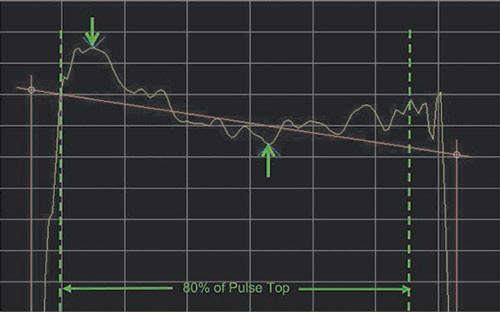
Figure 5 The pulse ripple measurement.
Other timing measurements include pulse width, repetition interval/duty cycle, peak amplitude, average ON power, average transmit power, droop and pulse top ripple. The ripple is defined as the difference between the peak positive and negative excursions from the best-fit line (which was already found to be the droop). This ripple, as seen in Figure 5, is expressed in percent of the pulse-top voltage.
Frequency and phase measurements
For CW pulses only, a frequency measurement can be made using the marker on a spectrum display, but this method has limitations due to the PRF lines that are an artifact of swept spectrum analysis and the difficulty of locating the center one to place the marker depending on the space interpolation and signal repeatability. The software uses a variety of methods to find the carrier frequency within pulses in preparation for automated measurement of phase and frequency parameters.
Pulse-to-pulse carrier phase difference is made using I/Q processing as other phase measurements. The accuracy of this measurement is subject to four major influences: signal-to-noise ratio, phase noise, estimation of the pulse rising edge, and finally the overshoot present on the pulse as measured.
The pulse-to-pulse frequency measurement is just like the corresponding phase measurement, except that the error effects are far less pronounced. Frequency measurement is a relative phase-change measurement made locally on the pulse, from which the frequency is calculated. Then the measured pulse frequency is compared to the reference pulse frequency, which was found locally within the first pulse.
Chirp measurements
There are specialized measurements required for verification of the performance of frequency chirped pulses. For simple time-of-flight pulsed CW radar, the main concern is that the timing parameters of the pulse be as designed. For chirp radar, the possible transmitted errors that will cause errors in the receiver can be much more subtle. While parameters such as pulse timing, center frequency, chirp frequency width and frequency errors across the chirp will all certainly cause problems when the transmitter adds these to the radiated signal, the phase errors across each pulse as well as from one pulse to another are the more subtle contributors to the success of chirped radar.
Long frame measurements (Multiple Pulses)
Measurement of a single pulse is not usually sufficient to assure transmitter performance. Many pulses can be measured. If there are differences from one pulse to another, this by itself can be used to diagnose problems that may be otherwise difficult to find.
The first view into such variations is the pulse table. When there are many pulses in one acquisition, the measured values can be arranged into a table where the numeric values of all measurements are calculated for each acquisition. The user can select which measurements will be shown in the table. Each column contains the results from one parameter displayed sequentially for all the pulses which were measured. A new column is added for each additional parameter selected by the user.
The results table shows variations in the pulse power of only about one tenth of a dB amongst the pulses. Even though this is only an extremely slight variation, it may be significant. To see if there is some regularity to the results, the trend of results is plotted. The trend plot plots one point for each pulse. This effectively removes the long time in between the pulses and gives a readable trend plot.

Figure 6 Plot of the trend of average ON power in a series of pulses.
Figure 6 shows such a plot for the results of Average ON Power of a series of pulses. There is a pronounced periodicity in the pulse power being produced by this transmitter. If the variations were random, then, as small as they are, they might well be ignored by the receiver. But a periodic variation may well produce false target information, so there is a need to find the nature of the periodicity as well as the cause.
The table of values is useful to manually see if there are anomalous readings for some pulses. The pulse trend plot graphically shows the character and magnitude of such variations. But to analyze these results and make a possible determination of the root cause for such variations requires further computations. The method provided is a Fast Fourier Transform (FFT) of the tabular pulse measurement results. Figure 7 shows the process.

Figure 7 The process of performing a FFT on measurement results of multiple pulses.
The drawing illustrates how the FFT might well have been from the previous trend plot. In this case, by analyzing just the ON samples of the Average ON measurements, and eliminating the OFF time samples, an FFT of the Average ON trend can be calculated. Here the 400 Hz primary power supply is modulating the transmit power. Having found a correlation between the variations and a possible cause, remedial action can now be taken.
Conclusion
The complicated pulses used in modern radar systems present significant measurement challenges in military and defense environments. The need for testing solutions extends throughout the lifecycle of a radar system from initial design, to production and through to signal monitoring. While there are somewhat different requirements at each phase, automated signal generation and test software help engineers make reliable and repeatable measurements.
Using AWG and signal creation software, signals can be inserted at any point in the radar chain to verify performance or to simulate a range of signal conditions. Using software together with oscilloscopes and spectrum analyzers, engineers can perform a full range of automated pulsed radar measurements including timing, frequency and phase, chirp and long frame measurements involving multiple pulses. No longer is it necessary for radar development teams to develop custom test benches to fully characterize and validate their designs due to a lack of suitable test solutions.